An Introduction To ngsReports
Christopher Ward
School of Biological Sciences, University of AdelaideHien To
Bioinformatics Hub, University of AdelaideStevie Pederson
Black Ochre Data Laboratories, Telethon Kids Institute, Adelaide, AustraliaDame Roma Mitchell Cancer Researc Laboratories, University of AdelaideJohn Curtin School of Medical Research, Australian National Universitystephen.pederson.au@gmail.com Source:
vignettes/ngsReportsIntroduction.Rmd
ngsReportsIntroduction.RmdIntroduction
The package ngsReports is designed to bolt into data
processing pipelines and produce combined plots for multiple FastQC
reports generated across an entire set of libraries or samples. The
primary functionality of the package is parsing FastQC reports, with
import methods also implemented for log files produced by tools as as
STAR, hisat2 and others. In addition to
parsing files, default plotting methods are implemented. Plots applied
to a single file will replicate the default plots from
FastQC1, whilst methods applied to multiple FastQC
reports summarise these and produce a series of custom plots.
Plots are produced as standard ggplot2 objects, with an interactive option available using plotly. As well as custom summary plots, tables of read counts and the like can also be easily generated.
Basic Usage
Using the Shiny App
In addition to the usage demonstrated below, a shiny app
has been developed for interactive viewing of FastQC reports. This can
be installed using:
remotes::install_github("UofABioinformaticsHub/shinyNgsreports")A vignette for this app will be installed with the
shinyNgsreports package.
The default report
In it’s simplest form, a default summary report can be generated
simply by specifying a directory containing the output from FastQC and
calling the function writeHtmlReport().
fileDir <- file.path("path", "to", "your", "FastQC", "Reports")
writeHtmlReport(fileDir)
This function will transfer the default template to the provided
directory and produce a single .html file containing
interactive summary plots of any FastQC output found in the directory.
FastQC output can be *fastqc.zip files or the same files
extracted as individual directories.
The default template is provided as
ngsReports_Fastqc.Rmd in the package directory . This
template can be easily modified and supplied as an alternate template to
the above function using your modified file as the template RMarkdown
file.
altTemplate <- file.path("path", "to", "your", "new", "template.Rmd")
writeHtmlReport(fileDir, template = altTemplate)
Advanced Usage
Classes Defined in the Package
The package ngsReports introduces two main
S4 classes:
-
FastqcData&FastqcDataList
FastqcData objects hold the parsed data from a
single report as generated by the stand-alone tool
FastQC. These are then extended into lists for more
than one file as a FastqcDataList. For most users, the
primary class of interest will be the FastqcDataList.
Loading FastQC Data Into R
To load a set of FastQC reports into R as a
FastqcDataList, specify the vector of file paths, then call
the function FastqcDataList(). In the rare case you’d like
an individual file, this can be performed by calling
FastqcData() on an individual file, or subsetting the
output from FastqcDataList() using the [[]]
operator as with any list object.
fileDir <- system.file("extdata", package = "ngsReports")
files <- list.files(fileDir, pattern = "fastqc.zip$", full.names = TRUE)
fdl <- FastqcDataList(files)
From here, all FastQC modules can be obtained as a
tibble (i.e. data.frame) using the function
getModule() and choosing one of the following modules:
-
Summary(The PASS/WARN/FAIL status for each module) Basic_StatisticsPer_base_sequence_qualityPer_sequence_quality_scoresPer_base_sequence_contentPer_sequence_GC_contentPer_base_N_contentSequence_Length_DistributionSequence_Duplication_LevelsOverrepresented_sequencesAdapter_ContentKmer_ContentPer_tile_sequence_quality
getModule(fdl[[1]], "Summary")## # A tibble: 12 × 3
## Filename Status Category
## <chr> <chr> <chr>
## 1 ATTG_R1.fastq PASS Basic Statistics
## 2 ATTG_R1.fastq FAIL Per base sequence quality
## 3 ATTG_R1.fastq WARN Per tile sequence quality
## 4 ATTG_R1.fastq PASS Per sequence quality scores
## 5 ATTG_R1.fastq FAIL Per base sequence content
## 6 ATTG_R1.fastq FAIL Per sequence GC content
## 7 ATTG_R1.fastq PASS Per base N content
## 8 ATTG_R1.fastq PASS Sequence Length Distribution
## 9 ATTG_R1.fastq FAIL Sequence Duplication Levels
## 10 ATTG_R1.fastq FAIL Overrepresented sequences
## 11 ATTG_R1.fastq FAIL Adapter Content
## 12 ATTG_R1.fastq FAIL Kmer ContentCapitalisation and spelling of these module names follows the default patterns from FastQC reports with spaces replaced by underscores. One additional module is available and taken directly from the text within the supplied reports
Total_Duplicated_Percentage
In addition, the read totals for each file in the library can be
obtained using readTotals(), which can be easily used to
make a table of read totals. This essentially just returns the first two
columns from getModule(x, "Basic_Statistics").
reads <- readTotals(fdl)The packages dplyr and pander can also be
extremely useful for manipulating and displaying imported data. To show
only the R1 read totals, you could do the following
library(dplyr)
library(pander)
reads %>%
    dplyr::filter(grepl("R1", Filename)) %>%
    pander(
        big.mark = ",",
        caption = "Read totals from R1 libraries",
        justify = "lr"
)| Filename | Total_Sequences |
|---|---|
| ATTG_R1.fastq | 24,978 |
| CCGC_R1.fastq | 22,269 |
| GACC_R1.fastq | 10,287 |
Generating Plots For One or More Fastqc Files
Plots created from a single FastqcData object will
resemble those generated by the FastQC tool, whilst those
created from a FastqcDataList will be combined summaries
across a library of files. In addition, all plots are able to be
generated as interactive plots using the argument
usePlotly = TRUE.
All FastQC modules have been enabled for plotting using default
S4 dispatch, with the exception of
Per_tile_sequence_quality.
Inspecting the PASS/WARN/FAIL Status of each module
The simplest of the plots is to summarise the
PASS/WARN/FAIL flags as produced by FastQC for
each module. This plot can be simply generated using
plotSummary()
plotSummary(fdl)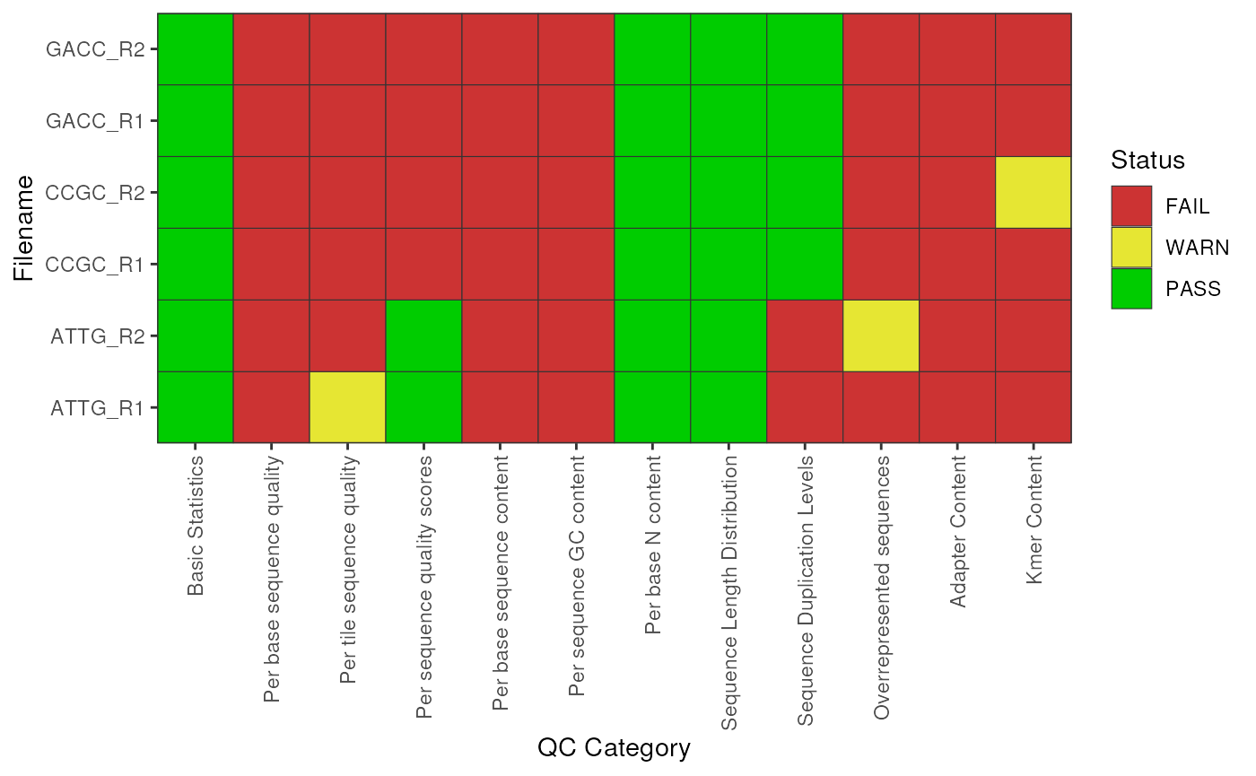
Default summary of FastQC flags.
Visualising Read Totals
The next most informative plot may be to summarise the total numbers
of reads in each associated Fastq file. By default, the number of
duplicated sequences from the Total_Duplicated_Percentage
module are shown, but this can be disabled by setting
duplicated = FALSE.
plotReadTotals(fdl)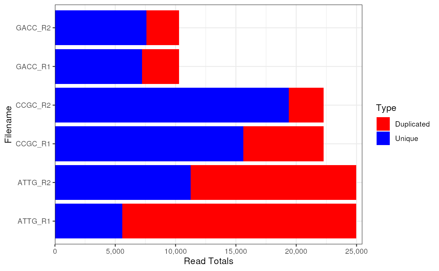
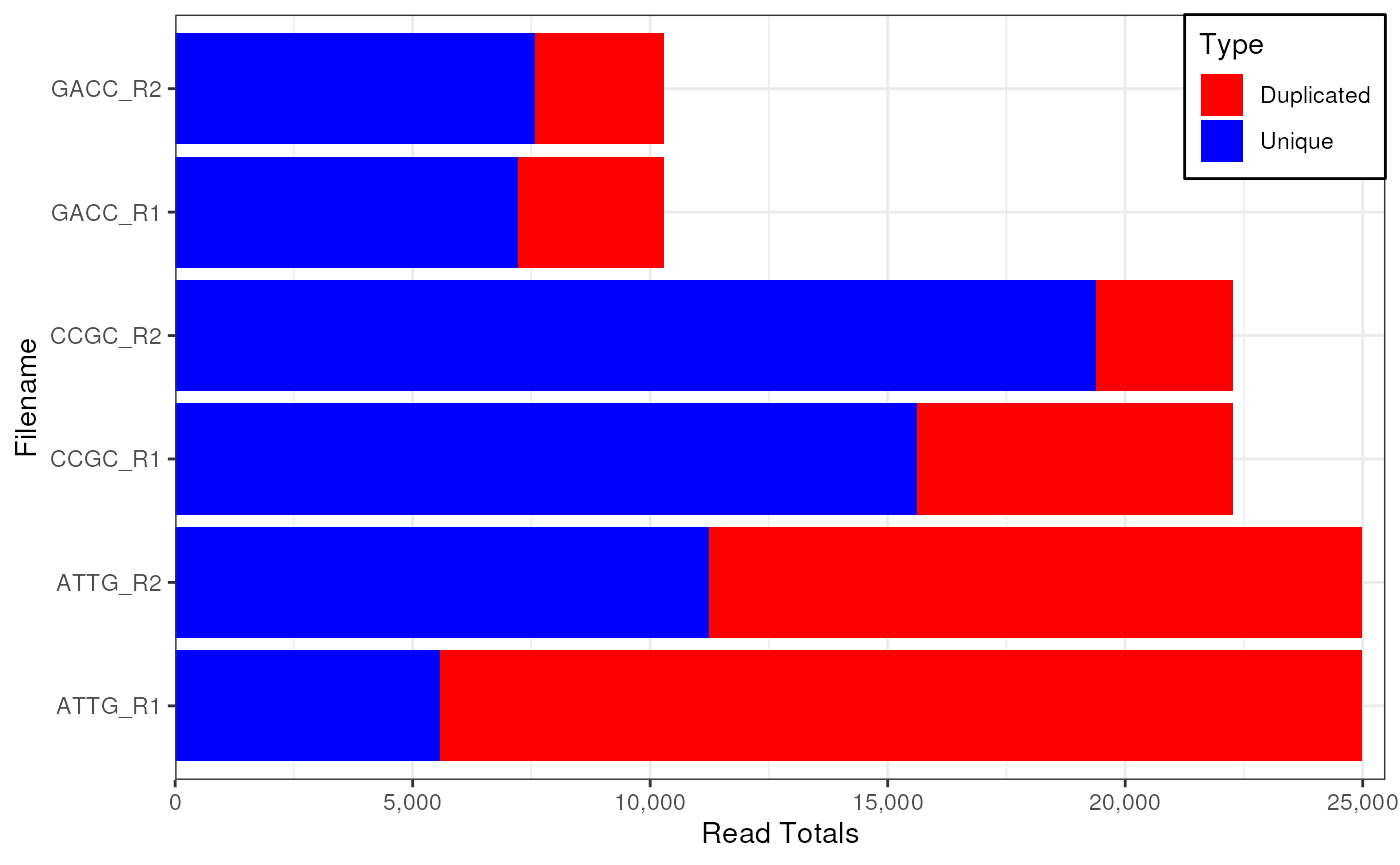
As these are ggplot2 objects, the output can be modified
easily using conventional ggplot2 syntax. Here we’ll move
the legend to the top right as an example.
plotReadTotals(fdl) +
    theme(
        legend.position = c(1, 1),
        legend.justification = c(1, 1),
        legend.background = element_rect(colour = "black")
    )
Per Base Sequence Qualities
Turning to the Per base sequence quality scores is the
next most common step for most researchers, and these can be obtained
for an individual file by selecting this as an element
(i.e. FastqcData object ) of the main
FastqcDataList object. This plot replicates the default
plots from a FastQC report.
plotBaseQuals(fdl[[1]])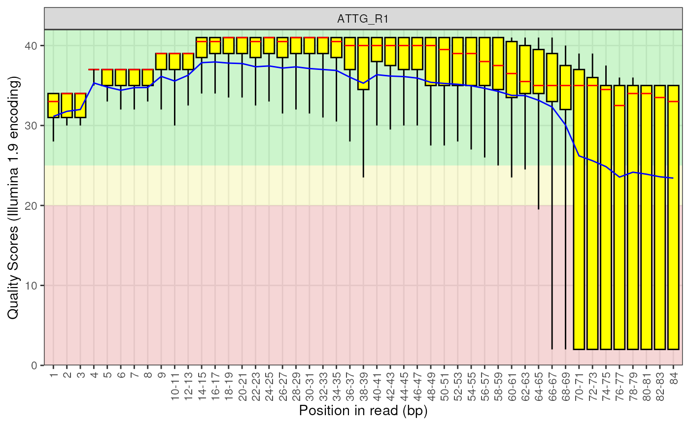
Example showing the Per_base_sequence_quality plot for a single FastqcData object.
When working with multiple FastQC reports, these are summarised as a heatmap using the mean quality score at each position.
plotBaseQuals(fdl)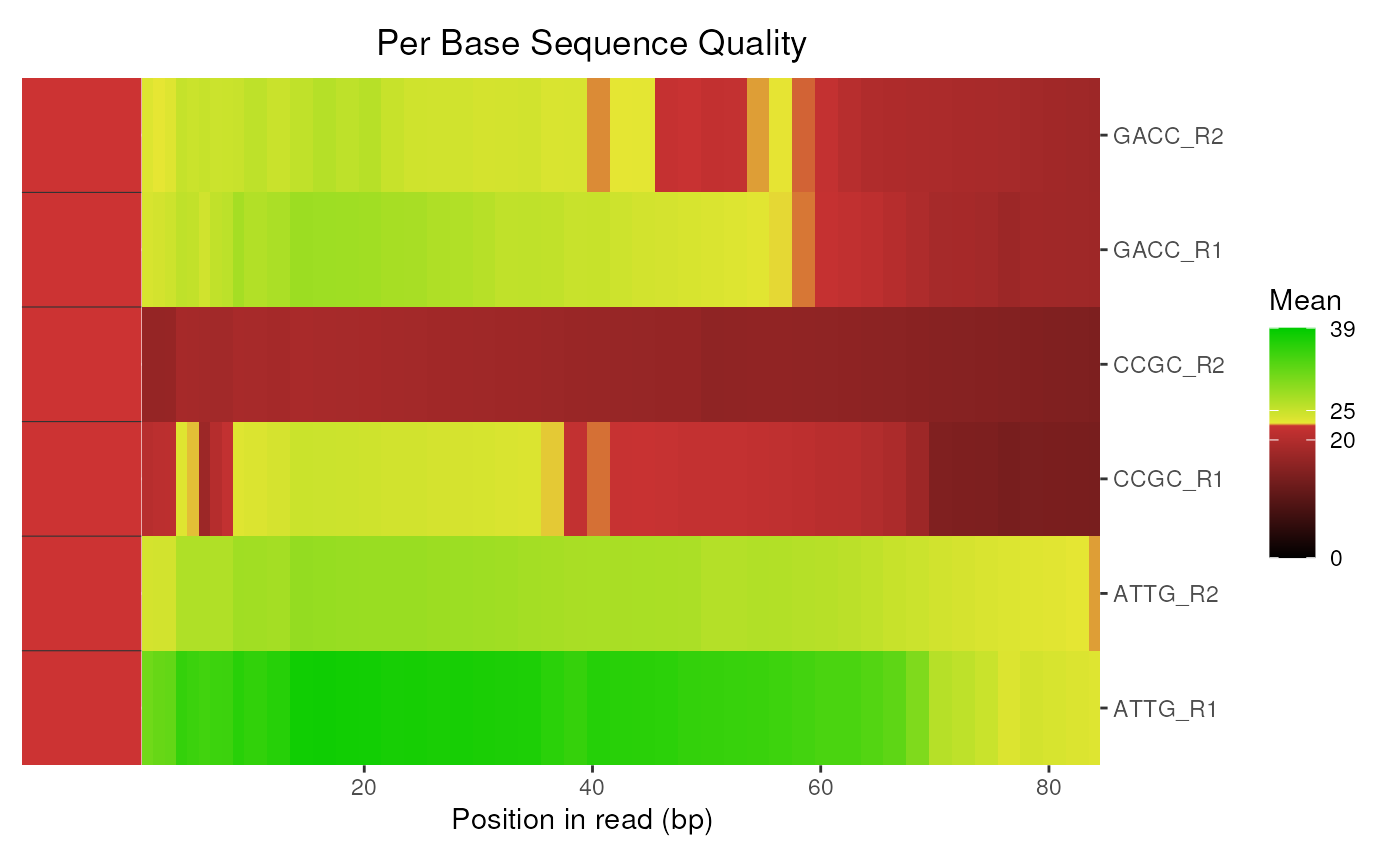
Example showing the Mean Per Base Squence Qualities for a set of FastQC reports.
Boxplots of any combinations can also be drawn from a
FastqcDataList by setting the argument
plotType = "boxplot". However, this may be not suitable for
datasets with a large number of libraries.
plotBaseQuals(fdl[1:4], plotType = "boxplot")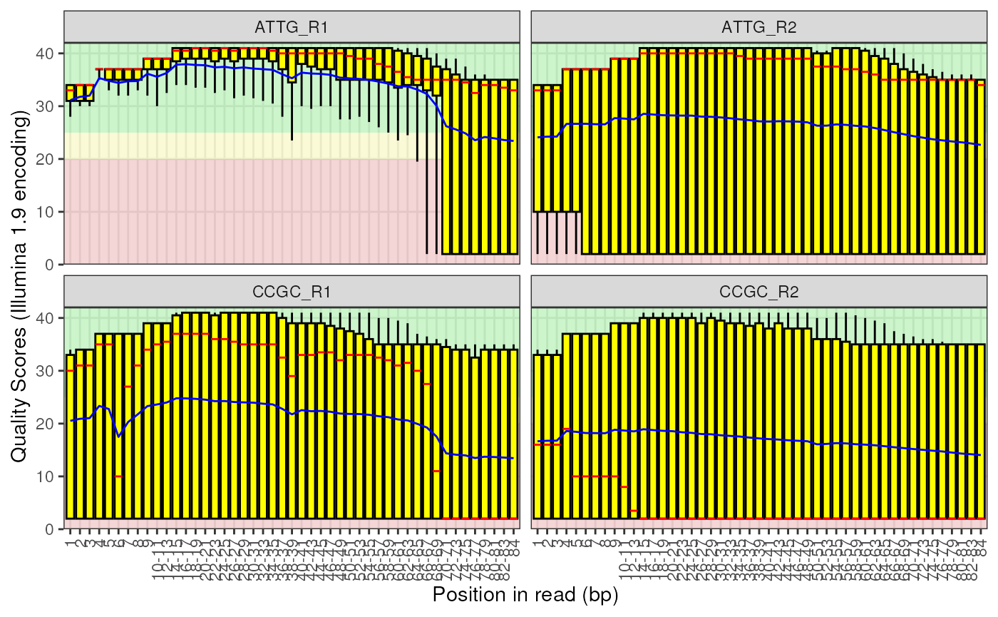
Mean Sequence Quality Per Read
Similarly, the Mean Sequence Quality Per Read plot can be generated
to replicate plots from a FastQC report by selecting the individual file
from the FastqcDataList object.
plotSeqQuals(fdl[[1]])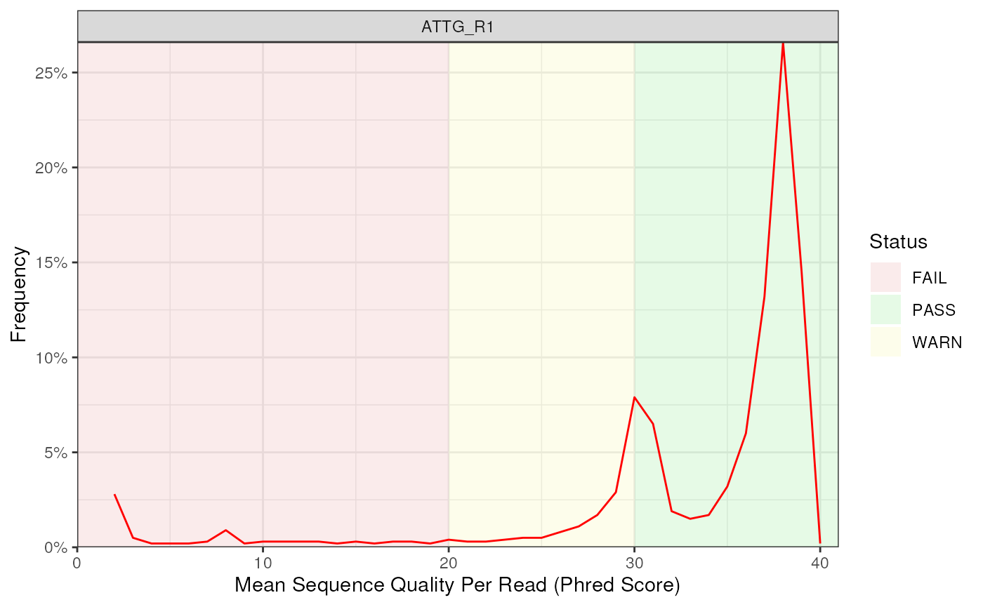
Example plot showing Per_sequence_quality_scores for an individual file.
A heatmap of mean sequence qualities can be generated when inspecting multiple reports.
plotSeqQuals(fdl)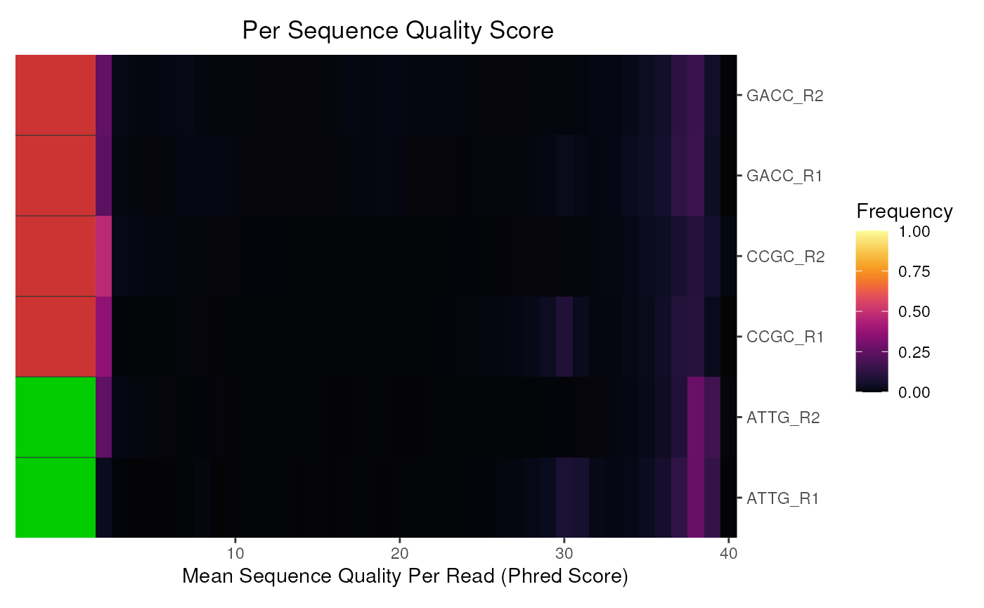
Example heatmaps showing Per_sequence_quality_scores for a set of files.
An alternative view may be to plot these as overlaid lines, which can
be simply done by setting plotType = "line". Again,
discretion should be shown when choosing this option for many
samples.
r2 <- grepl("R2", names(fdl))
plotSeqQuals(fdl[r2], plotType = "line")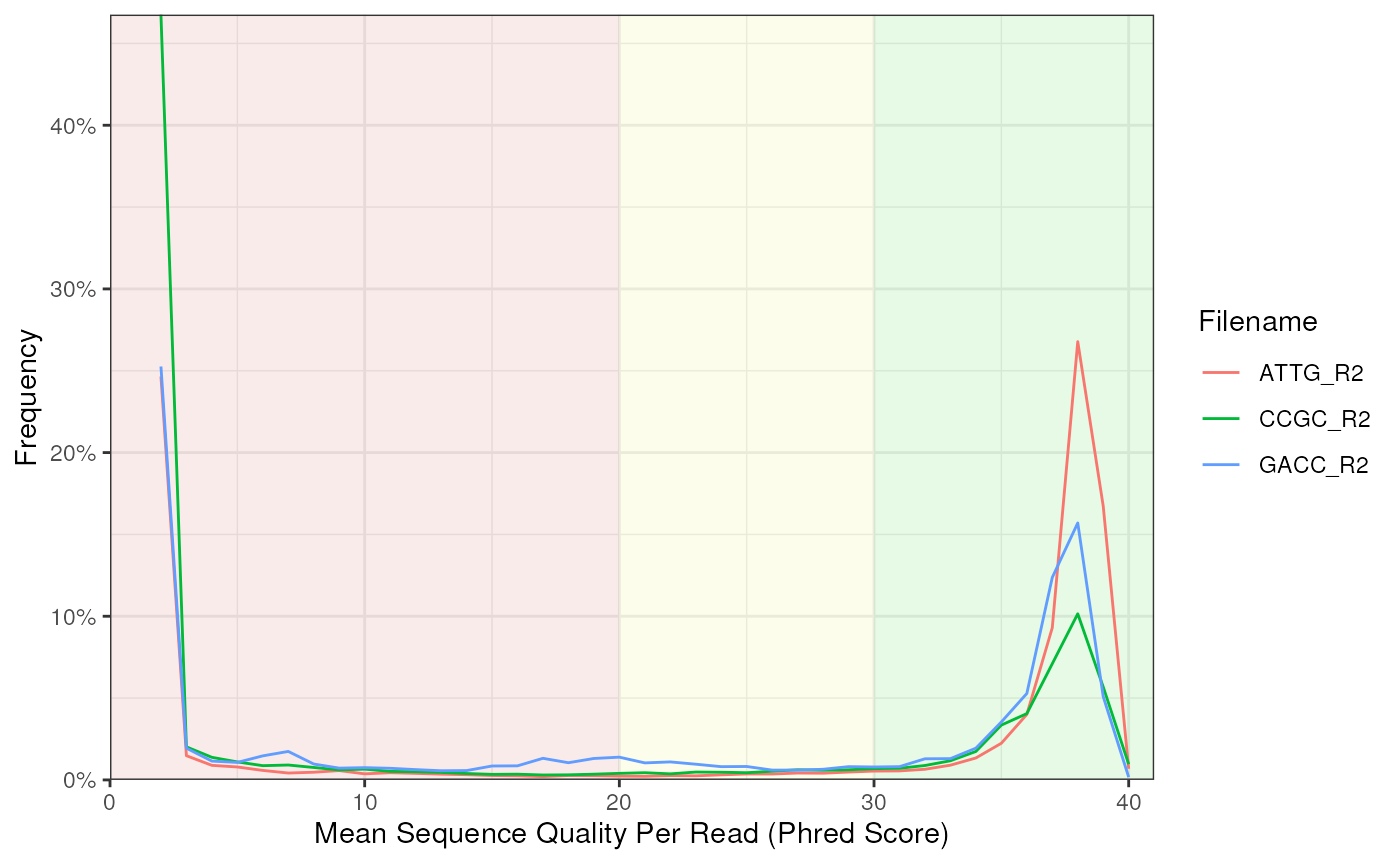
Per Base Sequence Content
The Per_base_sequence_content module can also be plotted
for an individual report with the layout being identical to that from
FastQC.
plotSeqContent(fdl[[1]])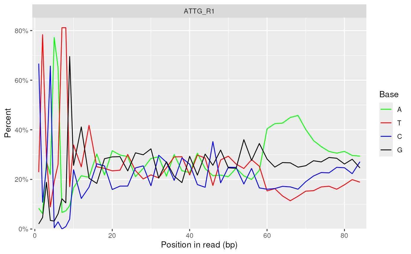
Individual Per_base_sequence_content plot
These are then combined across multiple files as a heatmap showing a
composite colour for each position. Colours are combined using
rgb() with A,C, G
and T being represented by green, blue, black and red
respectively.
plotSeqContent(fdl)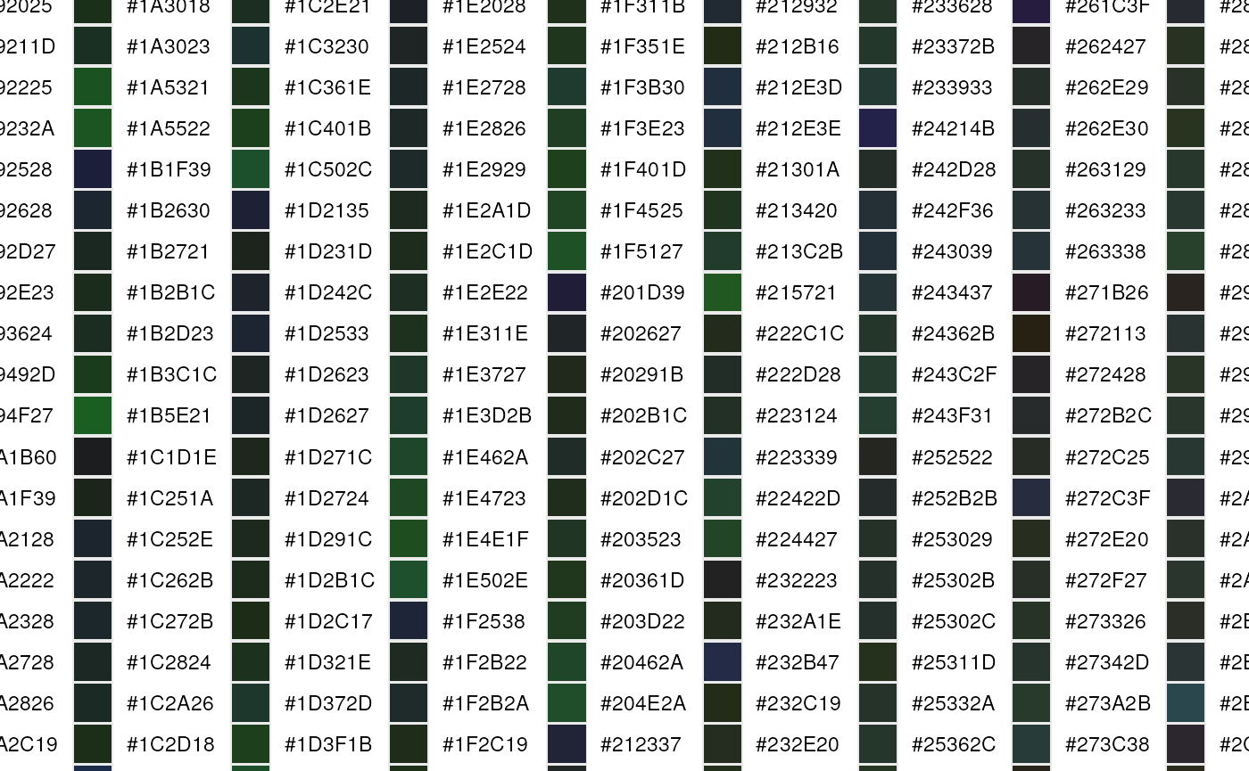
Combined Per_base_sequence_content plot
NB These plots can be very informative setting the
argument usePlotly = TRUE, however they can be slow to
render given the nature of how the package plotly renders
graphics.
Again, supplying multiple files and setting
plotType = "line" will replicate multiple individual plots
from the original FastQC reports. The argument nc is passed
to facet_wrap() from the package ggplot2 to
determine the number of columns in the final plot.
plotSeqContent(fdl[1:2], plotType = "line", nc = 1)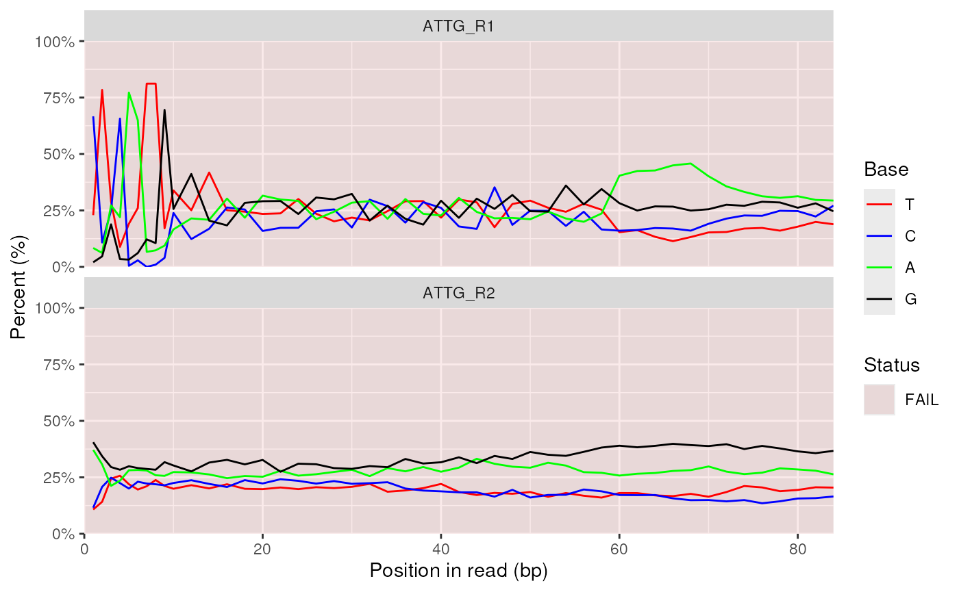
Adapter Content
Adapter content as identified by FastQC is also able to be plotted for an individual file.
plotAdapterContent(fdl[[1]]) 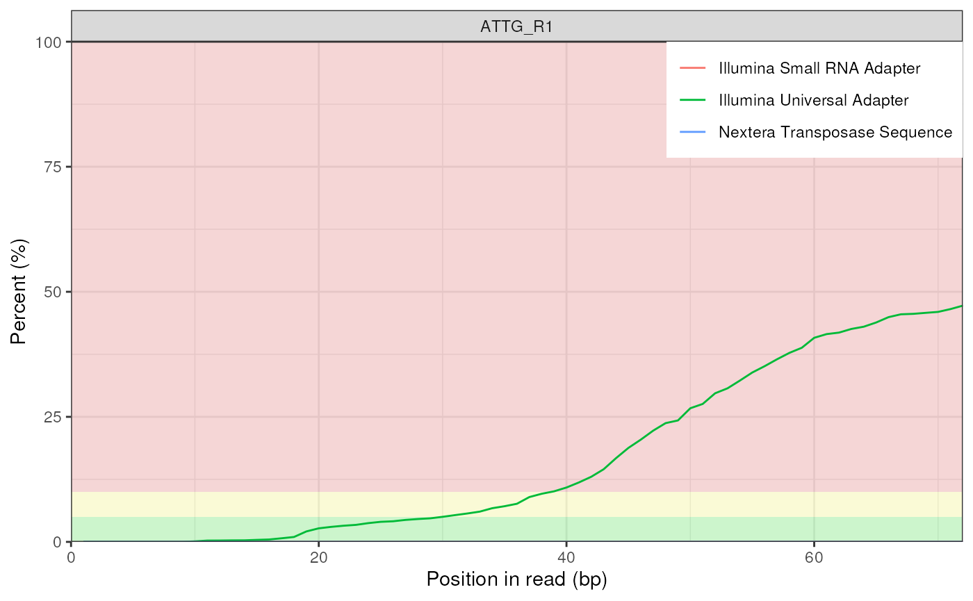
Adapter Content plot for a single FastQC report
When producing a heatmap across a set of FastQC reports, this will default to Total Adapter Content, instead of showing the individual adapter types.
plotAdapterContent(fdl)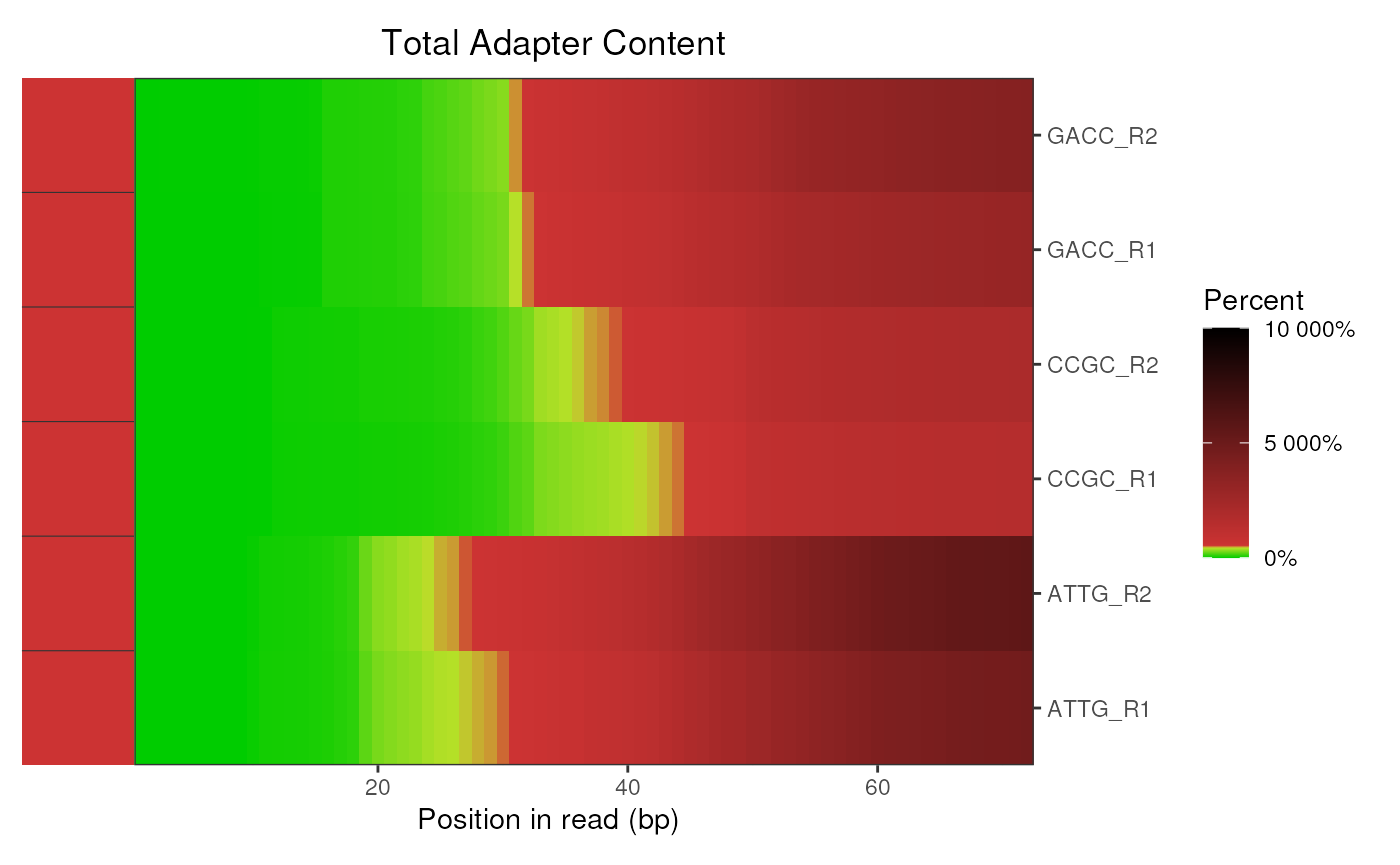
Heatmap showing Total Adapter Content by position across a set of FastQC reports
Sequence Duplication Levels
As with all modules, the Sequence Duplication Levels plot is able to be replicated for an individual file.
plotDupLevels(fdl[[1]])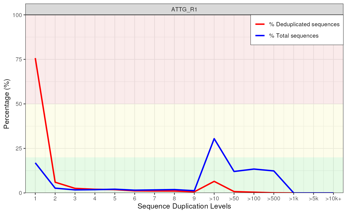
Example Sequence Duplication Levels plot for an individual file.
When plotting across multiple FastQC reports, duplication levels are
shown as a heatmap based on each default bin included in the initial
FastQC reports. By default, the plotted values are the “Pre”
de-duplication values. Note that values are converted to percentages
instead of read numbers to ensure comparability across files. In the
plot below, CCGC_R2 shows very low duplication levels,
whilst ATTG_R1 shows high levels of duplication. The
commonly observed ‘spikes’ around >10 are also evident
as the larger red blocks.
plotDupLevels(fdl)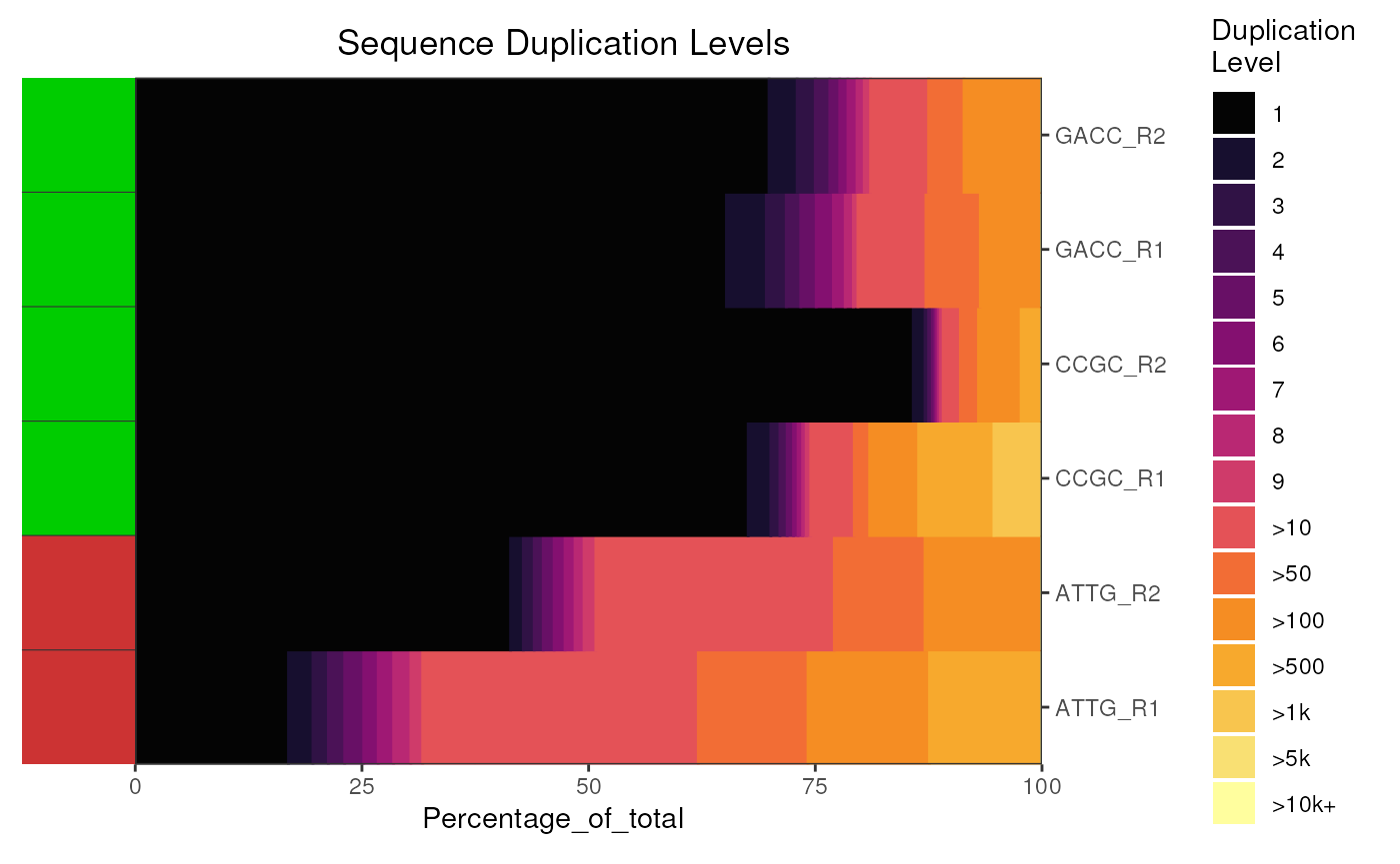
Sequence Duplication Levels for multiple files
GC content
The class TheoreticalGC
A selection of Theoretical GC content is supplied with the package in
the object gcTheoretical, which has been defined with the
additional S4 class TheoreticalGC. GC content
was calculated using scripts obtained from
https://github.com/mikelove/fastqcTheoreticalGC.
Available genomes and transcriptomes can be obtained using the function
gcAvail() on the object gcTheoretical and
specifying the type.
gcAvail(gcTheoretical, "Genome")## # A tibble: 24 × 4
## Name Group Source Version
## <chr> <chr> <chr> <chr>
## 1 Alyrata Plants JGI V1.0
## 2 Amellifera Animals UCSC apiMel2
## 3 Athaliana Plants TAIR Arapot11
## 4 Btaurus Animals UCSC bosTau8
## 5 Celegans Animals UCSC ce11
## 6 Cfamiliaris Animals UCSC canFam3
## 7 Dmelanogaster Animals UCSC dm6
## 8 Drerio Animals UCSC danRer10
## 9 Ecoli Bacteria NCBI 2008/08/05
## 10 Gaculeatus Other UCSC gasAcu1
## # ℹ 14 more rowsInspecting GC Content
As with all modules, data for an individual file replicates the
default plot from a FastQC report, but with one key difference. This is
that the Theoretical GC content has been provided in the object
gcTheoretical based on 100bp reads. This empirically
determined content is shown as the Theoretical GC content line.
plotGcContent(fdl[[1]], species = "Hsapiens", gcType = "Transcriptome")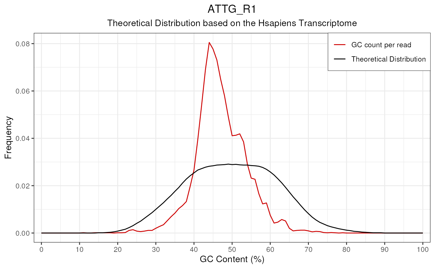
Example GC Content plot using the Hsapiens Transcriptome for the theoretical distribution.
Again, data is summarised as a heatmap when plotting across multiple reports, with the default value being the difference between the observed and the theoretical GC content.
plotGcContent(fdl)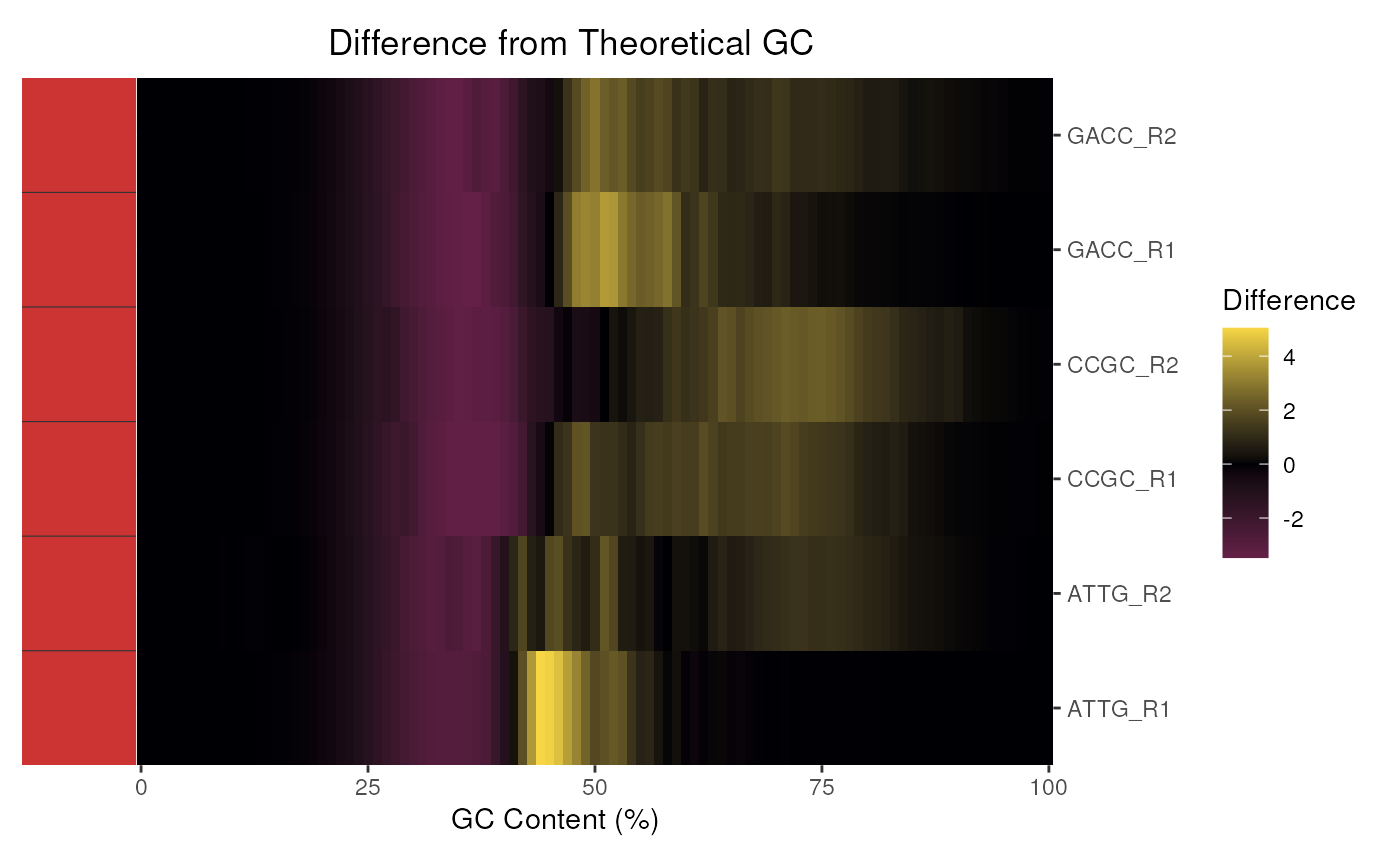
Example GC content showing the difference between observed and theoretical GC content across multiple files.
Line plots can also be produce an alternative viewpoint, with read totals displayed as percentages instead of raw counts.
plotGcContent(fdl, plotType = "line", gcType = "Transcriptome")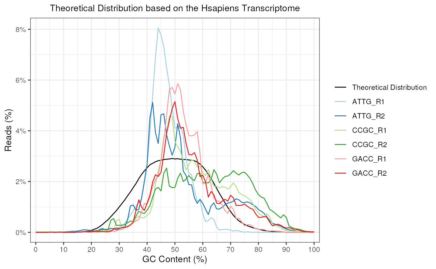
Example GC content plot represented as a line plot instead of a heatmap.
Customized theoretical GC content can be generated using input DNA sequences from a supplied fasta file.
faFile <- system.file(
    "extdata", "Athaliana.TAIR10.tRNA.fasta",
    package = "ngsReports")
plotGcContent(fdl, Fastafile = faFile, n = 1000)
Overrepresented Sequences
When inspecting the Overrepresented Sequence module, the top
ncan be plotted for an individual file, again broken down
by their possible source, and coloured based on their
WARN/FAIL status.
plotOverrep(fdl[[1]])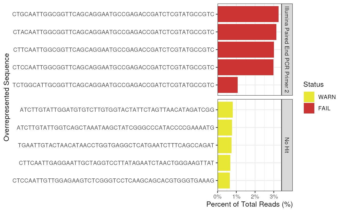
When applying this across multiple files, instead of identifying common sequences across a set of libraries, overrepresented sequences are summarised by their possible source as defined by FastQC.
plotOverrep(fdl)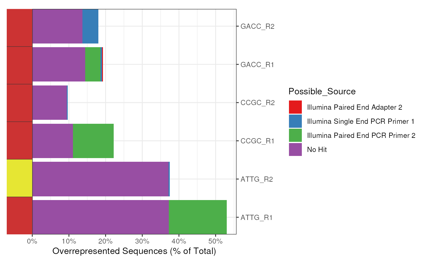
In addition to the above, the most abundant n
overrepresented sequences can be exported as a FASTA file for easy
submission to blast.
overRep2Fasta(fdl, n = 10)Importing Log Files
A selection of log files as produced by tools such as
STAR, hisat2, bowtie,
bowtie2 and picard duplicationMetrics, can be
easily imported using the importNgsLogs() function.
Tool can be specified by the user using the argument
type, however if no type is provided we will
attempt to auto-detect from the file’s structure. Note: only a single
log file type can be imported at any time.
The importNgsLogs() function currently supports log
files from the following tools.
Adapter removal and trimming
- AdapterRemoval
- cutadapt
- trimmomatic
Mapping and alignment
- bowtie
- bowtie2
- hisat2
- samtools flagstat
- STAR
- picard MarkDuplicates
Transcript/gene quantification
- featureCounts
Genome assembly
- BUSCO
- Quast
Adapter removal and trimming
fl <- c("Sample1.trimmomaticPE.txt")
trimmomaticLogs <- system.file("extdata", fl, package = "ngsReports")
df <- importNgsLogs(trimmomaticLogs)
df %>%
    dplyr::select("Filename", contains("Surviving"), "Dropped") %>%
    pander(
        split.tables = Inf,
        style = "rmarkdown",
        big.mark = ",",
        caption = "Select columns as an example of output from trimmomatic."
)| Filename | Both_Surviving | Forward_Only_Surviving | Reverse_Only_Surviving | Dropped |
|---|---|---|---|---|
| Sample1.trimmomaticPE.txt | 38243521 | 2791713 | 1464192 | 1663808 |
Mapping and alignment
Log file import
Bowtie log files can be parsed and imported
fls <- c("bowtiePE.txt", "bowtieSE.txt")
bowtieLogs <- system.file("extdata", fls, package = "ngsReports")
df <- importNgsLogs(bowtieLogs, type = "bowtie")
df %>%
    dplyr::select("Filename", starts_with("Reads")) %>%
    pander(
        split.tables = Inf,
        style = "rmarkdown",
        big.mark = ",",
        caption = "Select columns as an example of output from bowtie."
)| Filename | Reads_Processed | Reads_With_At_Least_One_Reported_Alignment | Reads_That_Failed_To_Align | Reads_With_Alignments_Suppressed_Due_To_-m |
|---|---|---|---|---|
| bowtiePE.txt | 42,867,915 | 21,891,058 | 20,748,783 | 228,074 |
| bowtieSE.txt | 440,372 | 193,962 | 246,410 | NA |
STAR log files can be parsed and imported
starLog <- system.file("extdata", "log.final.out", package = "ngsReports")
df <- importNgsLogs(starLog, type = "star")| Filename | Uniquely_Mapped_Reads_Number | Uniquely_Mapped_Reads_Percent |
|---|---|---|
| log.final.out | 68,471,490 | 85.84 |
The output of the samtools flagstat module can be parsed
and imported
flagstatLog <- system.file("extdata", "flagstat.txt", package = "ngsReports")
df <- importNgsLogs(flagstatLog, type = "flagstat")| Filename | QC-passed | QC-failed | flag |
|---|---|---|---|
| flagstat.txt | 67,405,447 | 0 | in total |
| flagstat.txt | 5,275,834 | 0 | secondary |
| flagstat.txt | 0 | 0 | supplementary |
| flagstat.txt | 0 | 0 | duplicates |
| flagstat.txt | 67,405,447 | 0 | mapped |
| flagstat.txt | 62,129,613 | 0 | paired in sequencing |
| flagstat.txt | 31,065,014 | 0 | read1 |
| flagstat.txt | 31,064,599 | 0 | read2 |
| flagstat.txt | 62,128,918 | 0 | properly paired |
| flagstat.txt | 62,128,918 | 0 | with itself and mate mapped |
| flagstat.txt | 695 | 0 | singletons |
| flagstat.txt | 0 | 0 | with mate mapped to a different chr |
| flagstat.txt | 0 | 0 | with mate mapped to a different chr (mapQ>=5) |
In addition to the files produced by the above alignment tools, the
output from Duplication Metrics (picard) can also be
imported. This is imported as a list with a tibble
containing the detailed output in the list element $metrics
and the histogram data included as the second elements.
sysDir <- system.file("extdata", package = "ngsReports")
fl <- list.files(sysDir, "Dedup_metrics.txt", full.names = TRUE)
dupMetrics <- importNgsLogs(fl, type = "duplicationMetrics", which = "metrics")
str(dupMetrics)
## tibble [1 × 10] (S3: tbl_df/tbl/data.frame)
## $ Library : chr "~/myExpt/2_alignedData/bams/Sample1.bam"
## $ Unpaired Reads Examined : int 93
## $ Read Pairs Examined : int 43490914
## $ Secondary Or Supplementary Rds: int 5366030
## $ Unmapped Reads : int 0
## $ Unpaired Read Duplicates : int 79
## $ Read Pair Duplicates : int 11494386
## $ Read Pair Optical Duplicates : int 642648
## $ Percent Duplication : num 0.264
## $ Estimated Library Size : int 69609522Plot log file imports
Summaries of log files from select mapping and alignment tools can be
plot using the function plotAlignemntSummary().
plotAlignmentSummary(bowtieLogs, type = "bowtie")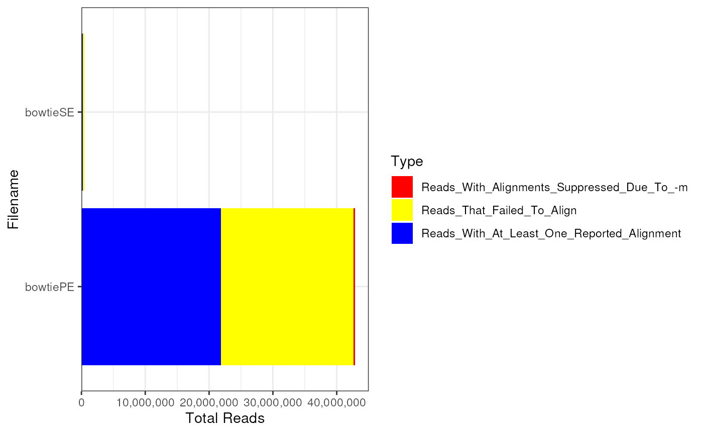
Example Bowtie logs for PE and SE sequencing
plotAlignmentSummary(starLog, type = "star")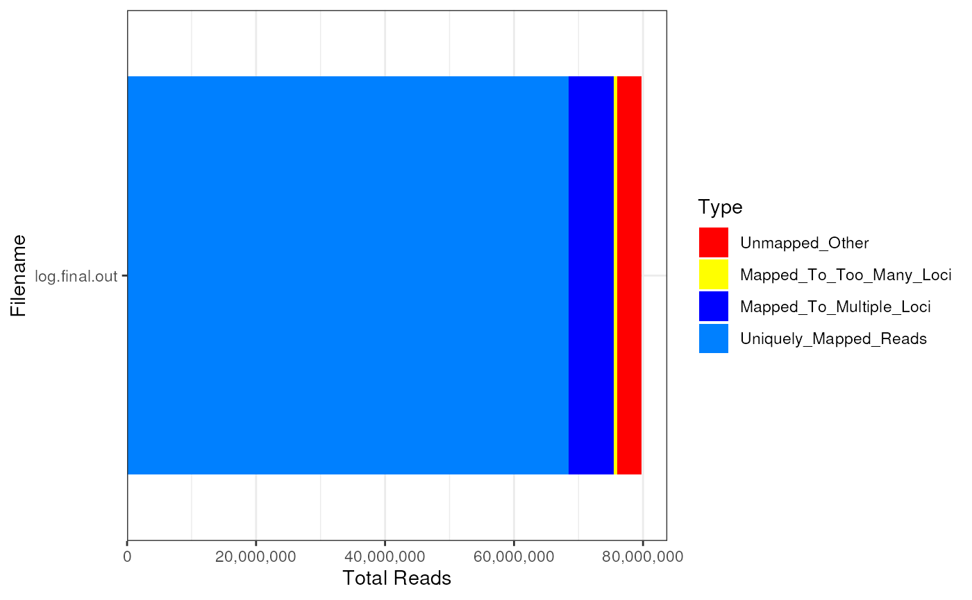
Example STAR aligner logs
Genome assembly
Assembly ‘completeness’ and summary statistic information from the
tools BUSCO and quast can also be plot using the function
plotAssemblyStats()
buscoLog <- system.file("extdata", "short_summary_Dmelanogaster_Busco.txt", package = "ngsReports")
plotAssemblyStats(buscoLog, type = "busco")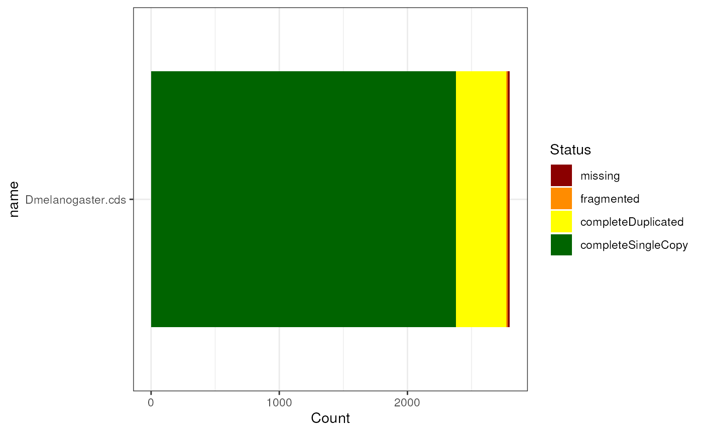
Example plot after running BUSCO v3 on the Drosophila melanogaster reference genome
fls <- c("quast1.tsv", "quast2.tsv")
quastLog <- system.file("extdata", fls, package = "ngsReports")
plotAssemblyStats(quastLog, type = "quast")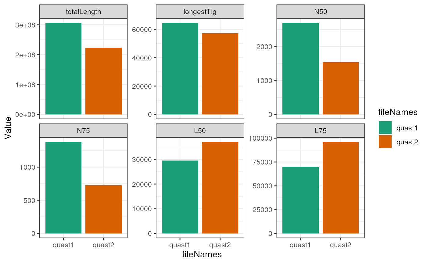
Example plot after running quast on two shortread assemblies
plotAssemblyStats(quastLog, type = "quast", plotType = "paracoord")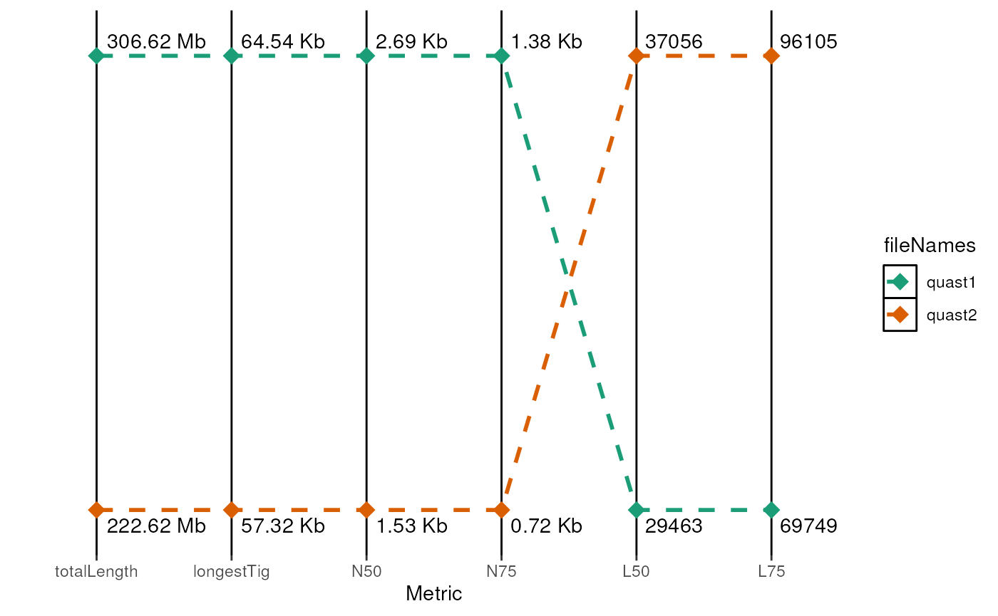
Example parallel coordinate plot after running quast on two shortread assemblies
Session info
## R version 4.5.2 (2025-10-31)
## Platform: x86_64-pc-linux-gnu
## Running under: Ubuntu 24.04.3 LTS
##
## Matrix products: default
## BLAS:   /usr/lib/x86_64-linux-gnu/openblas-pthread/libblas.so.3
## LAPACK: /usr/lib/x86_64-linux-gnu/openblas-pthread/libopenblasp-r0.3.26.so;  LAPACK version 3.12.0
##
## locale:
##  [1] LC_CTYPE=en_US.UTF-8       LC_NUMERIC=C
##  [3] LC_TIME=en_US.UTF-8        LC_COLLATE=en_US.UTF-8
##  [5] LC_MONETARY=en_US.UTF-8    LC_MESSAGES=en_US.UTF-8
##  [7] LC_PAPER=en_US.UTF-8       LC_NAME=C
##  [9] LC_ADDRESS=C               LC_TELEPHONE=C
## [11] LC_MEASUREMENT=en_US.UTF-8 LC_IDENTIFICATION=C
##
## time zone: UTC
## tzcode source: system (glibc)
##
## attached base packages:
## [1] stats     graphics  grDevices utils     datasets  methods   base
##
## other attached packages:
## [1] pander_0.6.6        dplyr_1.1.4         ngsReports_2.13.0
## [4] tibble_3.3.0        patchwork_1.3.2     ggplot2_4.0.0
## [7] BiocGenerics_0.56.0 generics_0.1.4      BiocStyle_2.38.0
##
## loaded via a namespace (and not attached):
##  [1] gtable_0.3.6        xfun_0.54           bslib_0.9.0
##  [4] htmlwidgets_1.6.4   lattice_0.22-7      vctrs_0.6.5
##  [7] tools_4.5.2         stats4_4.5.2        pkgconfig_2.0.3
## [10] data.table_1.17.8   RColorBrewer_1.1-3  S7_0.2.0
## [13] desc_1.4.3          S4Vectors_0.48.0    lifecycle_1.0.4
## [16] compiler_4.5.2      farver_2.1.2        stringr_1.6.0
## [19] textshaping_1.0.4   Biostrings_2.78.0   Seqinfo_1.0.0
## [22] htmltools_0.5.8.1   sass_0.4.10         yaml_2.3.10
## [25] lazyeval_0.2.2      plotly_4.11.0       pillar_1.11.1
## [28] pkgdown_2.2.0       crayon_1.5.3        jquerylib_0.1.4
## [31] tidyr_1.3.1         MASS_7.3-65         cachem_1.1.0
## [34] tidyselect_1.2.1    digest_0.6.37       stringi_1.8.7
## [37] purrr_1.2.0         bookdown_0.45       labeling_0.4.3
## [40] forcats_1.0.1       fastmap_1.2.0       grid_4.5.2
## [43] cli_3.6.5           magrittr_2.0.4      utf8_1.2.6
## [46] withr_3.0.2         scales_1.4.0        lubridate_1.9.4
## [49] timechange_0.3.0    rmarkdown_2.30      XVector_0.50.0
## [52] httr_1.4.7          ragg_1.5.0          zoo_1.8-14
## [55] evaluate_1.0.5      knitr_1.50          IRanges_2.44.0
## [58] viridisLite_0.4.2   rlang_1.1.6         ggdendro_0.2.0
## [61] Rcpp_1.1.0          glue_1.8.0          BiocManager_1.30.26
## [64] jsonlite_2.0.0      R6_2.6.1            systemfonts_1.3.1
## [67] fs_1.6.6