extraChIPs: Differential Signal Using Sliding Windows
Stevie Pederson
Black Ochre Data Laboratories, Telethon Kids Institute, Adelaide, AustraliaJohn Curtin School of Medical Research, Australian National Universitystephen.pederson.au@gmail.com Source:
vignettes/differential_signal_sliding.Rmd
differential_signal_sliding.Rmd
knitr::opts_chunk$set(message = FALSE, crop = NULL)Introduction
The GRAVI workflow, for
which this package is designed, uses sliding windows for differential
signal analysis using strategies defined in the package
csaw (Lun and Smyth 2016). The GRAVI workflow itself
extends to integrating multiple ChIP targets and external data sources,
and as such, this package introduces a handful of functions to simplify
and enable these analyses. Whilst many existing approaches refer to this
type of analysis as Differential Binding analysis, we prefer the term
Differential Signal Analysis as this more accurately captures
the range of ChIP targets which are likely to be investigated, such as
H3K27ac or similar.
The majority of examples below use heavily reduced datasets to
provide general guidance on using the functions. Some results may appear
trivial as a result, but will hopefully prove far more useful in a true
experimental context. All data, along with this vignette are available
here. In
order to replicate this vignette, please place all contents of the
data directory provided in this additional repository into
a directory named data in your own working directory.
It may also be worth noting that this vignette should run on a conventional laptop with no particularly large performance requirements. However, when following this workflow across an entire genome, memory requirements may exceed those of a standard laptop, and an HPC or high-performance workstation may be required.
Setup
Installation
In order to use the package extraChIPs and follow this
vignette, we recommend using the package BiocManager
(hosted on CRAN) to install all packages. Once BiocManager
is installed, the additional packages required for this vignette can
also be installed as shown below.
if (!"BiocManager" %in% rownames(installed.packages()))
  install.packages("BiocManager")
pkg <- c(
  "tidyverse", "Rsamtools", "csaw", "BiocParallel", "rtracklayer", "edgeR",
  "patchwork", "extraChIPs", "plyranges", "scales", "glue", "here", "quantro",
  "ggrepel", "BSgenome.Hsapiens.UCSC.hg19"
)
BiocManager::install(pkg, update = FALSE)
Once these packages are installed, we can load them easily
Data
All data for this vignette is expected to be in a sub-directory of the working directory named “data” (including “data/H3K27ac”), and all paths will be predicated on this. Please ensure you have all data in this location, obtained from here.
The data itself is ChIP-Seq data targeting the histone mark H3K27ac,
and is taken from the ZR-75-1 cell-line using data from the BioProject ,
Preprocessing was performed using the prepareChIPs
workflow, written in snakemake (Mölder et al. 2021) and all code is
available at https://github.com/smped/PRJNA509779. H3K27ac signal was
obtained under baseline (E2) and DHT-treated (E2DHT) conditions, with
alignments being to GRCh37. For this workflow, data has been subset to a
region found on chromosome 10 for simplicity.
A description of the samples can be found in the file
data/PRJNA509779.tsv. A pooled Input (IgG) sample was used
for the entire dataset and this accession is provided in a separate
column.
samples <- here("data", "PRJNA509779.tsv") %>%
  read_tsv() %>%
  dplyr::filter(target == "H3K27ac") %>%
  mutate(treatment = factor(treatment, levels = c("E2", "E2DHT")))
accessions <- unique(c(samples$accession, samples$input))
treat_colours <- c("steelblue", "red3", "grey")
names(treat_colours) <- c(levels(samples$treatment), "Input")
Differential Signal Analysis
Sliding Windows
The standard approach of tools such as DiffBind (Ross-Innes et
al. 2012) is to take a set of peaks, re-centre them, then set all
regions to be the same width. From there, data is passed to
edgeR (Chen, Lun, and Smyth 2016) or DESeq2
(Love, Huber, and Anders 2014) for analysis. This approach using
extraChIPs is demonstrated in a separate vignette, however,
this workflow instead focusses on a sliding window approach as per the
package csaw (Lun and Smyth 2016). The resultant
variable width regions can be particularly advantageous for
ChIP targets such as H3K27ac where regions marked by histone-acetylation
can vary greatly in size.
The starting point for differential signal analyses using
extraChIPs is to define a set of sliding windows across the
genome, then count reads from a set of bam files, defined as a
BamFileList. Commonly one or more IP input/control samples
is also produced during a ChIP-Seq experiment, and these should be
included at this stage of the analysis. The example files provided here
contain a small subset of reads from chromosome 10 across two
experimental conditions and one input sample, and we will define them
all as a BamFileList.
bfl <- here("data", "H3K27ac", glue("{accessions}.bam")) %>%
  BamFileList() %>%
  setNames(str_remove_all(names(.), ".bam"))
file.exists(path(bfl))
## [1] TRUE TRUE TRUE TRUE TRUE TRUE TRUESeqinfo objects are the foundation of working with
GRanges, so defining an object at the start of a workflow is good
practice. This is simply enabled with extraChIPs by using
defineSeqinfo() and specifying the appropriate genome.
sq <- defineSeqinfo("GRCh37")NB: It should also be noted that counting all reads
across a BamFileList using sliding windows, will
require >50Gb of RAM and will be beyond the capacity of most
laptops as of the time of writing. When working with complete datasets,
this particular step is best performed on an HPC or a similar
interactive server with a large amount of memory.
The approach taken below is to first define a set of sliding windows
across the genome, using the capabilities of csaw. After
counting reads across all windows, a set of pre-defined regions
where H3K27ac signal is confidently found, is then used guide the
function dualFilter(). This function will discard
low-signal windows, retaining only those a) above a minimum signal level
and b) with signal notably above that of any input samples. These
regions can be obtained from any external resource, or can even be taken
from macs2-defined peaks from the same samples. Here, the
set of regions was defined as those found when merging samples from each
treatment, in both treatments, with an FDR < 0.01. Importantly, our
analysis will not be restricted to these regions, but these will instead
guide dualFilter() as to the best regions to retain for
analysis.
First we can define our windows and count the alignments using the
existing capabilities and functions provided in the csaw
package. In the following, we’ll use a sliding window of 120bp and a
step size of 40bp, meaning each nucleotide is covered by 3 windows. In
addition, we’ll exclude blacklisted and grey-listed regions as provided
in the dataset. These can be obtained easily by using the
GreyListChIP package, which is beyond the scope of this
vignette, however, code for preparing the GreyList` is available here.
Fragment sizes for each sample were also estimated to be around
200nt.
greylist <- here("data", "chr10_greylist.bed") %>%
  import.bed(seqinfo = sq)
blacklist <- here("data", "chr10_blacklist.bed") %>%
  import.bed(seqinfo = sq)
rp <- readParam(
  pe = "none",
  dedup = TRUE,
  restrict = "chr10",
  discard = c(greylist, blacklist)
)
wincounts <- windowCounts(
  bam.files = bfl,
  spacing = 40,
  width = 120,
  ext = 200,
  filter = length(bfl),
  param = rp
)
seqlevels(wincounts) <- seqlevels(sq)
seqinfo(wincounts) <- sq
This produces a RangedSummarizedExperiment with windows
included which passed the minimum threshold of 7 total reads. We can
check which windows passed this threshold using
rowRanges()
rowRanges(wincounts)## GRanges object with 506538 ranges and 0 metadata columns:
## seqnames ranges strand
## <Rle> <IRanges> <Rle>
## [1] chr10 42491801-42491920 *
## [2] chr10 42491921-42492040 *
## [3] chr10 42494601-42494720 *
## [4] chr10 42495641-42495760 *
## [5] chr10 42495681-42495800 *
## ... ... ... ...
## [506534] chr10 99999641-99999760 *
## [506535] chr10 99999681-99999800 *
## [506536] chr10 99999721-99999840 *
## [506537] chr10 99999761-99999880 *
## [506538] chr10 99999801-99999920 *
## -------
## seqinfo: 25 sequences from GRCh37 genomeWe can also add some key information to the colData
element of this object, which will also be propagated to all downstream
objects.
colData(wincounts)## DataFrame with 7 rows and 4 columns
## bam.files totals ext rlen
## <character> <integer> <integer> <integer>
## SRR8315186 /home/steviep/github.. 267342 200 75
## SRR8315187 /home/steviep/github.. 307383 200 75
## SRR8315188 /home/steviep/github.. 288965 200 75
## SRR8315189 /home/steviep/github.. 296764 200 75
## SRR8315190 /home/steviep/github.. 325211 200 75
## SRR8315191 /home/steviep/github.. 283745 200 75
## SRR8315192 /home/steviep/github.. 361835 200 75
colData(wincounts) <- colData(wincounts) %>%
  as_tibble(rownames = "accession") %>%
  left_join(samples, by = "accession") %>%
  dplyr::select(
    accession, all_of(colnames(colData(wincounts))), target, treatment
  ) %>%
  mutate(
    target = str_replace_na(target, "Input"),
    treatment = str_replace_na(treatment, "Input") %>%
      as.factor()
  ) %>%
  DataFrame(row.names = .$accession)
A density plot can be simply drawn of these counts, with the vast majority of windows receiving very low counts, due to the nature of transcription factor binding, where long stretches are unbound. The windows with higher counts tend to be associated with the samples targeting a transcription factor (TF), as seen in the two treatment group samples.
plotAssayDensities(wincounts, colour = "treatment", trans = "log1p") +
  theme_bw() +
  scale_colour_manual(values = treat_colours)
Filtering of Sliding Windows
After counting all reads in the sliding genomic windows, the next
step is to discard windows for which counts are unlikely to represent
true signal from our ChIP target. The strategy employed in
extraChIPs uses a set of pre-defined regions to
automatically set thresholds based on 1) counts strongly above the
counts from the input sample, and 2) the windows with the overall
highest signal. Thresholds are determined such that a proportion
(e.g. q = 0.5) of the windows which overlap one of the
supplied consensus peaks will be returned. Higher values for
q will return more windows, however many of these will tend
to only marginally overlap a peak in one of the tail regions, and these
will most likely be covered by neighbouring windows. Experience has
shown that values such as q = 0.5 tend to return a
considerable proportion of windows containing true signal from the ChIP
target. Higher values will tend to return more sliding windows where the
edges overlap the tails of the guide regions.
The we can pass these to the function dualFilter() which
utilises the strategy described above. On large datasets, this can be
quite time-consuming, as can the initial counting step. Multiple
alternative filtering strategies are also provided by the package
csaw and these can be accessed using
?csaw::filterWindows
guide_regions <- here("data", "H3K27ac", "H3K27ac_chr10.bed") %>%
  import.bed(seqinfo = sq)
filtcounts <- dualFilter(
  x = wincounts, bg = "SRR8315192", ref = guide_regions, q = 0.6
)
Thus we have reduced our initial set of 506,538 sliding windows to
the 23,417 windows most likely to contain true signal from our ChIP
target. The returned object will by default contain counts
and logCPM assays, with the complete library sizes used for
the calculation of logCPM values. Similarly, the input
sample is no longer included in the data object, although
additional columns can easily be added to the returned object using any
number of strategies.
dim(wincounts)## [1] 506538 7
dim(filtcounts)## [1] 23417 6
assays(filtcounts)## List of length 2
## names(2): counts logCPMThe rowData element of the returned object will contain
a logical column indicating where each specific retained window
overlapped one of the supplied consensus peaks.
rowRanges(filtcounts)## GRanges object with 23417 ranges and 1 metadata column:
## seqnames ranges strand | overlaps_ref
## <Rle> <IRanges> <Rle> | <logical>
## [1] chr10 42862921-42863040 * | TRUE
## [2] chr10 42862961-42863080 * | TRUE
## [3] chr10 42863001-42863120 * | TRUE
## [4] chr10 42863041-42863160 * | TRUE
## [5] chr10 42863081-42863200 * | TRUE
## ... ... ... ... . ...
## [23413] chr10 99895121-99895240 * | TRUE
## [23414] chr10 99895161-99895280 * | TRUE
## [23415] chr10 99895201-99895320 * | TRUE
## [23416] chr10 99895241-99895360 * | TRUE
## [23417] chr10 99895281-99895400 * | TRUE
## -------
## seqinfo: 25 sequences from GRCh37 genomeInitial Visualisation
We can once again check our signal distributions, this time on the logCPM values. We can also check the samples using a PCA plot, again colouring the points by treatment group and adding labels, which will repel by default if the points are shown.
A <- plotAssayDensities(filtcounts, assay = "logCPM", colour = "treatment") +
  scale_colour_manual(values = treat_colours) +
  theme_bw()
B <- plotAssayPCA(filtcounts, "logCPM", colour = "treatment", label = "accession") +
  scale_colour_manual(values = treat_colours) +
  theme_bw()
A + B +
  plot_layout(guides = "collect") + plot_annotation(tag_levels = "A")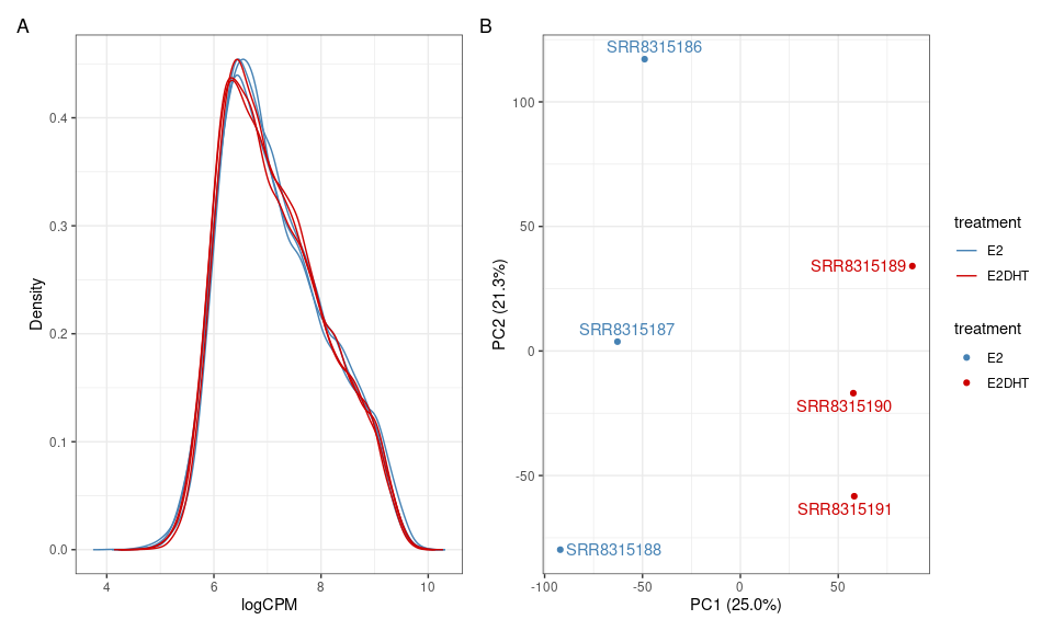
A) Densities for logCPM values across all samples after discarding
windows less likely to contain H3K27ac signal using
dualFilter() B) PCA plot based on the logCPM assay
Another common QC step is Relative Log-Expression (RLE) (Gandolfo and Speed 2018). In the following, we first inspect the RLE across the entire dataset, followed by RLE grouping within treatments. This can be particularly useful when distributions vary significantly between treatment groups, such as may occur with a cytoplasmic to nuclear shift by a given ChIP target. Here, however, there is minimal difference between the two approaches as H3K27ac signal tends to be broadly consistent between these treatment groups.
a <- plotAssayRle(filtcounts, assay = "logCPM", fill = "treat") +
  geom_hline(yintercept = 0, linetype = 2, colour = "grey") +
  scale_fill_manual(values = treat_colours) +
  ggtitle("RLE: Across All Samples") +
  theme_bw()
b <- plotAssayRle(
  filtcounts, assay = "logCPM", fill = "treat", rle_group = "treat"
) +
  geom_hline(yintercept = 0, linetype = 2, colour = "grey") +
  scale_fill_manual(values = treat_colours) +
  ggtitle("RLE: Within Treatment Groups") +
  theme_bw()
a + b + plot_layout(guides = "collect") +
  plot_annotation(tag_levels = "A")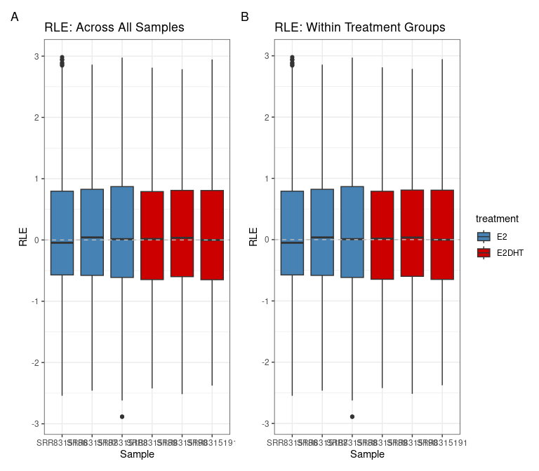
RLE plots (A) across all samples and (B) with values calculated within treatment groups
Statistical Testing
Multiple methods are enabled in the package extraChIPs
via the function fitAssayDiff(), with the possibility of
incorporating any additional normalisation strategies from external
packages. The two basic strategies are 1) Quasi-Likelihood Fits (Lund et
al. 2012) and 2) limma-trend (Law et al. 2014). The first
approach (method = “qlf”) uses counts along with any of the
normalisation strategies from edgeR::calcNormFactors(), and
setting the normalisation method to “none” is the equivalent of
library-size normalisation, which replicates the default normalisation
strategy from DiffBind (Ross-Innes et al. 2012). If choosing to
normalise within treatment groups, a factor can be provided via
the groups argument, essentially adding this as an option for all
methods provided in edgeR::calcNormFactors(). The second
method (method = “lt”) is specifically for logCPM values and these can
be provided as output by dualFilter() or may be normalised
using any number of additional methods. In addition to the above
methods, a range-based
(McCarthy and Smyth 2009) can be specified by providing a value to the
fc or lfc arguments, which removes any need
for post-hoc filtering and correctly controls the FDR, unlike
post-hoc filtering based on a fold-change threshold.
Here, we’ll initially fit our data using Quasi-Likelihood Fits,
library-size normalisation and setting a change in signal beyond the
range of
20% as being of interest. By default, the returned object, would be a
SummarizedExperiment object containing the results from
model fitting in the rowData() element. However, setting
asRanges = TRUE will simply return the set of GRanges along
with the testing results as a stand-alone object.
X <- model.matrix(~treatment, data = colData(filtcounts))
fit_gr <- fitAssayDiff(filtcounts, design = X, fc = 1.2, asRanges = TRUE)
Merging Windows
After an analysis has been performed, values contained in the output
will be estimated signal (logCPM), estimated change
(logFC) with both raw and adjusted p-values for all sliding
windows. Given the dependency of neighbouring windows, any adjusted
p-values will not be appropriate and a merging of overlapping and/or
neighbouring windows should be performed. Multiple csaw
methods are wrapped using mergeByCol(),
mergeBySig() with minor changes to the returned object,
such as the inclusion of the representative range in the column
keyval_range.
For this vignette, we’ll merge using the asymptotically exact harmonic mean p-value, which can also be used for merging dependent p-values (Wilson 2019). This approach tests H0: no -value in the set of p-values is significant. When merging windows using the harmonic mean p-values, instead of values from a representative window, weighted averages for the expression and logFC estimates are returned using the weights . A representative window, corresponding to the original window with the lowest p-value is returned.
results_gr <- mergeByHMP(fit_gr, inc_cols = "overlaps_ref", merge_within = 120) %>%
  addDiffStatus(drop = TRUE)
arrange(results_gr, hmPValue)[1:5]
## GRanges object with 5 ranges and 10 metadata columns:
## seqnames ranges strand | n_windows n_up n_down
## <Rle> <IRanges> <Rle> | <integer> <integer> <integer>
## [1] chr10 79257441-79258720 * | 30 3 0
## [2] chr10 43689241-43690160 * | 21 2 0
## [3] chr10 74008161-74008760 * | 13 2 0
## [4] chr10 63858841-63859040 * | 3 1 0
## [5] chr10 63859401-63859760 * | 7 1 0
## overlaps_ref keyval_range logCPM logFC hmPValue
## <logical> <GRanges> <numeric> <numeric> <numeric>
## [1] TRUE chr10:79257761-79257880 7.01563 1.82950 2.08382e-12
## [2] TRUE chr10:43689681-43689800 6.49125 1.78743 8.37664e-09
## [3] TRUE chr10:74008441-74008560 6.48379 1.81692 9.27730e-09
## [4] TRUE chr10:63858881-63859000 5.98361 1.75311 6.38262e-07
## [5] TRUE chr10:63859601-63859720 5.98163 1.82260 1.02640e-06
## hmPValue_fdr status
## <numeric> <factor>
## [1] 1.49827e-09 Increased
## [2] 2.22346e-06 Increased
## [3] 2.22346e-06 Increased
## [4] 1.14728e-04 Increased
## [5] 1.47597e-04 Increased
## -------
## seqinfo: 24 sequences from GRCh37 genomeIn the above, we returned 19 ranges which we might consider using the significance threshold = 0.05. As is common, we can assess our results using an MA plot. However, given that testing is performed using sliding windows and merging windows using the harmonic mean will introduce a bias, we can check using the complete set of sliding windows and the final set of merged windows. Any bias present in our data will be visible when using the sliding windows, whilst our final results can be inspected using the merged windows.
A <- fit_gr %>%
  as_tibble() %>%
  ggplot(aes(logCPM, logFC)) +
  geom_point(alpha = 0.6) +
  geom_smooth(se = FALSE, method = "loess") +
  geom_label(
    aes(label = label),
    data = . %>%
      summarise(
        n = dplyr::n(),
        logCPM = max(logCPM) - 0.15 * diff(range(logCPM)),
        logFC = max(logFC) - 0.05 * diff(range(logFC)),
        label = glue("{comma(n)}\nSliding Windows")
      )
  ) +
  ylim(range(fit_gr$logFC)) +
  ggtitle("MA Plot: All Retained Sliding Windows")
B <- results_gr %>%
  as_tibble() %>%
  mutate(`FDR < 0.05` = hmPValue_fdr < 0.05) %>%
  ggplot(aes(logCPM, logFC)) +
  geom_point(aes(colour = `FDR < 0.05`), alpha = 0.6) +
  geom_smooth(se = FALSE, method = "loess") +
  geom_label_repel(
    aes(label = range, colour = `FDR < 0.05`),
    data = . %>% dplyr::filter(hmPValue_fdr == min(hmPValue_fdr)),
    show.legend = FALSE
  ) +
  geom_label(
    aes(label = label),
    data = . %>%
      summarise(
        n = dplyr::n(),
        logCPM = max(logCPM) - 0.15 * diff(range(logCPM)),
        logFC = max(fit_gr$logFC) - 0.05 * diff(range(fit_gr$logFC)),
        label = glue("{comma(n)}\nMerged Windows")
      )
  ) +
  scale_colour_manual(values = c("black", "red")) +
  ylim(range(fit_gr$logFC)) +
  ggtitle("MA Plot: Merged Windows")
A + B + plot_annotation(tag_levels = "A")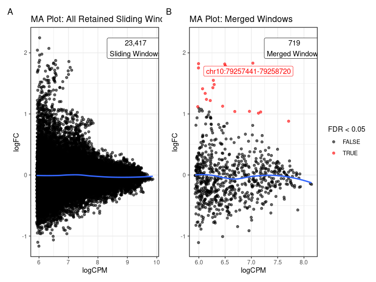
MA Plots using A) all sliding windows (after filtering before merging) and B) the final set of merged windows. The most highly ranked merged window is also labelled in the set of merged windows. Blue lines represent a loess curve through the data.
A particularly beneficial feature of this approach is that the final ranges will be of highly variable width, with this select region of chromosome 10 producing merged windows ranging from 120bp to 18.88kb, as may be expected for H3K27ac signal.
Alternative Normalisation Approaches
Using Library Size normalisation, as above, is a conservative approach and other methods such as RLE (Love, Huber, and Anders 2014) or TMM (Robinson and Oshlack 2010) may be appropriate. However, these methods assume that signal distributions are drawn from the same distributions across all samples, which unlike most RNA-Seq, is not always able to be safely assumed for ChIP-Seq data. An example may be when an transcription factor is primarily cytoplasmic in one treatment group, before being translocated to the nucleus in another treatment. The Androgen Receptor (AR) is a common example of this behaviour.
Whilst H3K27ac signal should remain approximately constant between
these two treatments, we can easily check for differences in data
distributions as well as any GC-bias. The package quantro
(Hicks and Irizarry 2015) provides a useful test for any difference in
medians as well as differences in the underlying distributions.
set.seed(100)
qtest <- assay(filtcounts, "counts") %>%
  quantro(groupFactor = filtcounts$treatment, B = 1e3)
qtest
## quantro: Test for global differences in distributions
## nGroups: 2
## nTotSamples: 6
## nSamplesinGroups: 3 3
## anovaPval: 0.49809
## quantroStat: 0.19728
## quantroPvalPerm: 0.68Here, no differences were evident across median values (ANOVA p = 0.498) or between distributions (p = 0.68) and as such, TMM/RLE normalisation across all samples may be appropriate.
TMM Normalisation
To perform an analysis using TMM-normalisation, we can simply specify
this using the argument norm = "TMM" when calling
fitAssayDiff()
tmm_gr <- fitAssayDiff(
  filtcounts, design = X, fc = 1.2, norm = "TMM", asRanges = TRUE
)
tmm_results <- mergeByHMP(tmm_gr, inc_cols = "overlaps_ref", merge_within = 120) %>%
  addDiffStatus(drop = TRUE)
table(tmm_results$status)
##
## Unchanged Increased
## 698 21As might be expected, the results are highly concordant, with
TMM-normalisation providing a moderate improvement in statistical power,
returning 21 windows with evidence of differential signal, instead of
the initial 19. Any of the normalisation methods taken by
edgeR::calcNormFactors() can be used here.
If a difference in distributions is found between groups, the
normalisation step can be set to only occur within treatment groups, by
passing the grouping column name to the groups = argument.
However, this may exaggerate differences between groups and may
introduce false positives, so should only be used when compelling
evidence exists and the underlying biology supports this.
Checking MA-plots shows that the very slight negative bias in higher-signal windows when using library size normalisation, as seen above, was lessened after TMM normalisation.
tmm_gr %>%
  as_tibble() %>%
  ggplot(aes(logCPM, logFC)) +
  geom_point(alpha = 0.6) +
  geom_smooth(se = FALSE, method = "loess") +
  ggtitle("MA Plot: TMM Normalisation")
If choosing more nuanced normalisation strategies, passing any offset
matrices can be simply done using the offset argument,
which will over-ride any other normalisation settings.
Mapping of Windows
Mapping to Genes
Once the changes in signal for our given ChIP target have been
determined, a common next step is to assess which genes are likely to be
impacted. Whilst no definitive, single methodology exists for this
process, the function mapByFeature() offers an intuitive
approach, taking into account any previously defined regulatory
features. These regulatory features may be defined by simple proximity
to TSS regions, by histone marks, downloaded from external repositories
or any other possibility. Whilst these features can improve the
precision of mapping, even without these this function can still enable
a useful assignment of target gene to binding event.
The process undertaken inside mapByFeature() is a
sequential checking of each range’s association with regulatory features
and the most likely target as a result. These steps are:
-
Check for any HiC interactions
- All genes which directly overlap an interaction anchor are considered part of the regulatory network for that interaction, and as such, all genes associated with both anchors are assigned to a peak which overlaps a HiC Interaction
-
Check for any overlaps with a promoter
- All genes regulated by that promoter are assigned as regulatory
targets. By default, this is by direct promoter/gene overlap
(
prom2gene = 0)
- All genes regulated by that promoter are assigned as regulatory
targets. By default, this is by direct promoter/gene overlap
(
-
Check for any overlaps with an enhancer
- Peaks which overlap an enhancer are assigned to all genes
within the distance specified by
enh2gene(default = 100kb)
- Peaks which overlap an enhancer are assigned to all genes
within the distance specified by
-
Check for genes with no previous mappings
- Peaks with no previous mappings are assigned to all
directly overlapping genes, or the nearest gene within a
specified distance (default
gr2gene= 100kb)
- Peaks with no previous mappings are assigned to all
directly overlapping genes, or the nearest gene within a
specified distance (default
If no promoters, enhancers or long-range interactions are supplied, all genes will be simply mapped to ChIP-Seq regions using step 4.
A GTF of annotations can be used, with the following being the genes,
transcripts and exons from chr10, taken from Gencode
v43. Whilst this example relies on this format, any additional
resource such as an EnsDb or TxDb object could
easily be used. Here, we’ll load the data then split into a
GRangesList with separate elements for genes, transcripts
and exons.
gencode <- here("data/gencode.v43lift37.chr10.annotation.gtf.gz") %>%
  import.gff() %>%
  filter_by_overlaps(GRanges("chr10:42354900-100000000")) %>%
  split(.$type)
seqlevels(gencode) <- seqlevels(sq)
seqinfo(gencode) <- sq
Now we’ve loaded our gene annotations at multiple levels, we can
easily define Transcription Start Sites (TSS) using transcript
definitions and the function reduceMC(). This function is
an extension of GenomicRanges::reduce() which retains all
supplied columns in the mcols() element by collapsing these
into CompressedList columns, and simplifying to vectors
where possible.
tss <- gencode$transcript %>%
  resize(width = 1, fix = "start") %>%
  select(gene_id, ends_with("name")) %>%
  reduceMC(min.gapwidth = 0)
Checking the TSS for PPIF shows we have one site which 3 transcripts start at, along with two more unique to specific transcripts.
## GRanges object with 3 ranges and 3 metadata columns:
##       seqnames    ranges strand |              gene_id       gene_name
##          <Rle> <IRanges>  <Rle> |      <CharacterList> <CharacterList>
##   [1]    chr10  81107225      + | ENSG00000108179.14_6            PPIF
##   [2]    chr10  81107256      + | ENSG00000108179.14_6            PPIF
##   [3]    chr10  81107414      + | ENSG00000108179.14_6            PPIF
##                  transcript_name
##                  <CharacterList>
##   [1] PPIF-205,PPIF-203,PPIF-201
##   [2]                   PPIF-204
##   [3]                   PPIF-202
##   -------
##   seqinfo: 25 sequences from GRCh37 genome
We can also add the TSS overlap status to our set of results
tmm_results$tss <- overlapsAny(tmm_results, tss)Next we’ll want to map our regions to genes. To use the methods
available in mapByFeature() let’s define a set of
promoters. First we’ll create a promoter for each transcript, then we
can merge any overlapping promoters using reduceMC().
(Setting simplify = FALSE avoids an issue in this subset of
genes where one gene has multiple IDs, and helps retain a 1:1 mapping
between IDs and genes.) Importantly, this will give a set of promoters
which are unique and non-overlapping but with variable width and with
the complete set of transcripts that may be regulated by the promoter
listed. As can be seen, 4 potential promoter regions are found for
CRTAC1
promoters <- gencode$transcript %>%
    select(gene_id, ends_with("name")) %>%
    promoters(upstream = 2500, downstream = 500) %>%
    reduceMC(simplify = FALSE)
tail(promoters)
## GRanges object with 6 ranges and 3 metadata columns:
## seqnames ranges strand |
## <Rle> <IRanges> <Rle> |
## [1] chr10 99609056-99612055 - |
## [2] chr10 99635155-99638154 - |
## [3] chr10 99643500-99646805 - |
## [4] chr10 99695536-99698535 - |
## [5] chr10 99770595-99773594 - |
## [6] chr10 99789879-99793085 - |
## gene_id gene_name
## <CharacterList> <CharacterList>
## [1] ENSG00000227356.2_10 GOLGA7B-DT
## [2] ENSG00000265398.1 AL139239.1
## [3] ENSG00000095713.14_13,ENSG00000095713.14_13 CRTAC1,CRTAC1
## [4] ENSG00000095713.14_13 CRTAC1
## [5] ENSG00000095713.14_13 CRTAC1
## [6] ENSG00000095713.14_13,ENSG00000095713.14_13 CRTAC1,CRTAC1
## transcript_name
## <CharacterList>
## [1] GOLGA7B-DT-201
## [2] AL139239.1-201
## [3] CRTAC1-205,CRTAC1-206
## [4] CRTAC1-204
## [5] CRTAC1-201
## [6] CRTAC1-203,CRTAC1-202
## -------
## seqinfo: 25 sequences from GRCh37 genome
tmm_results <- mapByFeature(
  tmm_results, genes = gencode$gene,
  prom = select(promoters, gene_id, gene_name)
)
tmm_results %>% filter(hmPValue_fdr < 0.05) %>% arrange(hmPValue)
## GRanges object with 21 ranges and 13 metadata columns:
## seqnames ranges strand | n_windows n_up n_down
## <Rle> <IRanges> <Rle> | <integer> <integer> <integer>
## [1] chr10 79257441-79258720 * | 30 3 0
## [2] chr10 43689241-43690160 * | 21 2 0
## [3] chr10 74008161-74008760 * | 13 2 0
## [4] chr10 63858841-63859040 * | 3 1 0
## [5] chr10 63859401-63859760 * | 7 1 0
## ... ... ... ... . ... ... ...
## [17] chr10 79307081-79307960 * | 20 2 0
## [18] chr10 74014401-74015360 * | 22 3 0
## [19] chr10 90615361-90615640 * | 4 2 0
## [20] chr10 63696921-63697240 * | 6 3 0
## [21] chr10 74878001-74878360 * | 7 3 0
## overlaps_ref keyval_range logCPM logFC hmPValue
## <logical> <GRanges> <numeric> <numeric> <numeric>
## [1] TRUE chr10:79257761-79257880 7.02793 1.85621 6.20766e-13
## [2] TRUE chr10:43689681-43689800 6.51086 1.81157 4.45187e-09
## [3] TRUE chr10:74008441-74008560 6.49275 1.84270 5.07996e-09
## [4] TRUE chr10:63858881-63859000 5.99257 1.77724 4.03575e-07
## [5] TRUE chr10:63859601-63859720 5.99366 1.84777 6.37775e-07
## ... ... ... ... ... ...
## [17] TRUE chr10:79307441-79307560 6.45271 1.15247 0.000563495
## [18] TRUE chr10:74015201-74015320 6.14440 1.26391 0.000592892
## [19] TRUE chr10:90615361-90615480 5.97947 1.14308 0.000804490
## [20] TRUE chr10:63697121-63697240 6.00058 1.11473 0.001074487
## [21] TRUE chr10:74878201-74878320 6.19539 1.05769 0.001437350
## hmPValue_fdr status tss gene_id gene_name
## <numeric> <character> <logical> <CharacterList> <CharacterList>
## [1] 4.46331e-10 Increased FALSE ENSG00000156113.25_17 KCNMA1
## [2] 1.21750e-06 Increased FALSE ENSG00000198915.12_14 RASGEF1A
## [3] 1.21750e-06 Increased FALSE ENSG00000166295.9_6 ANAPC16
## [4] 7.25426e-05 Increased FALSE ENSG00000150347.17_12 ARID5B
## [5] 9.17121e-05 Increased FALSE ENSG00000150347.17_12 ARID5B
## ... ... ... ... ... ...
## [17] 0.0236827 Increased FALSE ENSG00000156113.25_17 KCNMA1
## [18] 0.0236827 Increased FALSE ENSG00000289506.2_2 ENSG00000289506
## [19] 0.0304436 Increased FALSE ENSG00000152766.6_8 ANKRD22
## [20] 0.0386278 Increased FALSE ENSG00000150347.17_12 ARID5B
## [21] 0.0492121 Increased FALSE ENSG00000166321.14_7 NUDT13
## -------
## seqinfo: 25 sequences from GRCh37 genomeSo now we have our regions showing differential signal, along with which gene they are most likely to be impacting, and whether they directly overlap the TSS. This can all be summarised into a single MA-plot for presentation of final results.
status_colours <- c(Unchanged = "grey70", Increased = "red3", Decreased = "royalblue")
tmm_results %>%
  as_tibble() %>%
  ggplot(aes(logCPM, logFC, colour = status, shape = tss)) +
  geom_point() +
  geom_label_repel(
    aes(label = label),
    data = . %>%
      arrange(hmPValue) %>%
      dplyr::slice(1:20) %>%
      mutate(
        label  = vapply(gene_name, paste, character(1), collapse = "; ") %>%
          str_trunc(30)
      ),
    fill = "white", alpha = 0.6, show.legend = FALSE
  ) +
  scale_colour_manual(values = status_colours) +
  scale_shape_manual(values = c(19, 21))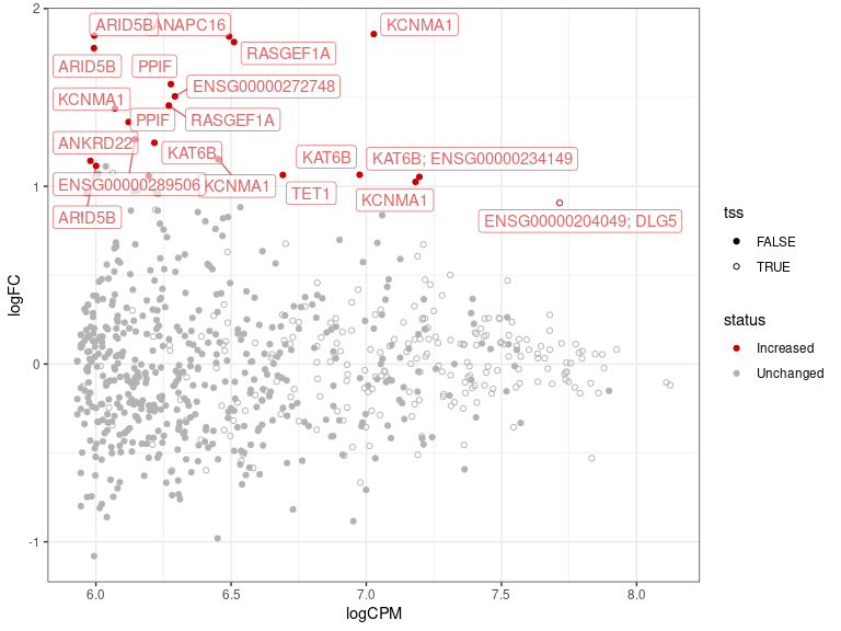
MA-plot with the top 20 regions by significance labelled according to the most likely gene influenced by the detected signal. Regions which directly overlap a TSS are shown as empty circles
Mapping to Regions
In addition to which gene is likely to be directly impacted by the
detected signal, knowing which type of regulatory region signal was
observed in is another question commonly asked of ChIP-Seq data. The
function deinfeRegions() takes, gene-, transcript- and
exon-level information from an annotation source and creates unique
region annotations across the genome. These are for in hierarchical
order as: 1) Promoters, 2) Upstream Promoters, 3) Exons, 4) Introns, 5)
Proximal Intergenic and, 6 Distal Intergenic regions.
regions <- defineRegions(
  genes = gencode$gene, transcripts = gencode$transcript, exons = gencode$exon
)
regions
## GRangesList object of length 6:
## $promoter
## GRanges object with 1491 ranges and 5 metadata columns:
## seqnames ranges strand | region
## <Rle> <IRanges> <Rle> | <character>
## [1] chr10 42644498-42647497 * | Promoter (-2500/+500)
## [2] chr10 42678287-42681286 * | Promoter (-2500/+500)
## [3] chr10 42702938-42705937 * | Promoter (-2500/+500)
## [4] chr10 42729924-42732923 * | Promoter (-2500/+500)
## [5] chr10 42735669-42738668 * | Promoter (-2500/+500)
## ... ... ... ... . ...
## [1487] chr10 99695536-99698535 * | Promoter (-2500/+500)
## [1488] chr10 99770595-99773594 * | Promoter (-2500/+500)
## [1489] chr10 99789879-99793085 * | Promoter (-2500/+500)
## [1490] chr10 99891881-99894913 * | Promoter (-2500/+500)
## [1491] chr10 99920140-99923543 * | Promoter (-2500/+500)
## gene_id gene_name
## <CharacterList> <CharacterList>
## [1] ENSG00000229485.1_5 KSR1P1
## [2] ENSG00000237592.2_5 IGKV1OR10-1
## [3] ENSG00000271650.1_7 ENSG00000271650
## [4] ENSG00000264398.1 AL031601.1
## [5] ENSG00000290458.1_2 ENSG00000290458
## ... ... ...
## [1487] ENSG00000095713.14_13 CRTAC1
## [1488] ENSG00000095713.14_13 CRTAC1
## [1489] ENSG00000095713.14_13 CRTAC1
## [1490] ENSG00000166024.14_8 R3HCC1L
## [1491] ENSG00000166024.14_8 R3HCC1L
## transcript_id
## <CharacterList>
## [1] ENST00000446298.1_2
## [2] ENST00000442306.2_2
## [3] ENST00000605702.1_2
## [4] ENST00000580460.1
## [5] ENST00000622823.4_3
## ... ...
## [1487] ENST00000413387.5_4
## [1488] ENST00000309155.3_5
## [1489] ENST00000370597.8_11,ENST00000370591.6_9
## [1490] ENST00000370584.7_7,ENST00000298999.8_8
## [1491] ENST00000370586.6_5,ENST00000613938.4_5,ENST00000612478.4_2,...
## transcript_name
## <CharacterList>
## [1] KSR1P1-201
## [2] IGKV1OR10-1-201
## [3] ENST00000605702
## [4] AL031601.1-201
## [5] ENST00000622823
## ... ...
## [1487] CRTAC1-204
## [1488] CRTAC1-201
## [1489] CRTAC1-203,CRTAC1-202
## [1490] R3HCC1L-203,R3HCC1L-201
## [1491] R3HCC1L-204,R3HCC1L-206,R3HCC1L-205,...
## -------
## seqinfo: 25 sequences from GRCh37 genome
##
## ...
## <5 more elements>We can now use the function bestOverlap() to assign each
window with ChIP-Seq signal to the region which it shows the greatest
overlap, setting this as a factor which reflects the hierarchy with
which the regions were defined.
tmm_results$bestOverlap <- bestOverlap(tmm_results, regions) %>%
  factor(levels = names(regions))
filter(tmm_results, hmPValue_fdr < 0.05, bestOverlap == "promoter")
## GRanges object with 2 ranges and 14 metadata columns:
## seqnames ranges strand | n_windows n_up n_down
## <Rle> <IRanges> <Rle> | <integer> <integer> <integer>
## [1] chr10 76779561-76780200 * | 14 4 0
## [2] chr10 79623321-79635960 * | 314 13 0
## overlaps_ref keyval_range logCPM logFC hmPValue
## <logical> <GRanges> <numeric> <numeric> <numeric>
## [1] TRUE chr10:76779721-76779840 6.21638 1.244849 0.000194483
## [2] TRUE chr10:79630321-79630440 7.71543 0.906496 0.000100434
## hmPValue_fdr status tss
## <numeric> <character> <logical>
## [1] 0.00932221 Increased FALSE
## [2] 0.00515801 Increased TRUE
## gene_id gene_name
## <CharacterList> <CharacterList>
## [1] ENSG00000156650.14_17 KAT6B
## [2] ENSG00000204049.1_8,ENSG00000151208.17_11 ENSG00000204049,DLG5
## bestOverlap
## <factor>
## [1] promoter
## [2] promoter
## -------
## seqinfo: 25 sequences from GRCh37 genomeGiven the region column contains nicely formateed output, we can also use this
Visualisation of Results
Pie Charts
Now that we’ve assigned each window to a genomic regions, we can use
plotPie() to view the distribution of ChIP-Seq signal
within these regions. First we’ll define a consistent colour palette for
these regions in all plots.
region_colours <- hcl.colors(length(reg_levels), "Viridis", rev = TRUE)
names(region_colours) <- reg_levels
Labels produced using plotPie() use the
glue() syntax and are able to access the summarised data
using N as the overall total number of sites. as well as
.data[[fill]] to access data in the column selected to fill
the pie segments. Totals and percentages within each segment are
accessible using n and p respectively as these
are columns within the internal data.frame formed when
creating the plot. External formatting functions such as
comma(), percent() or
str_to_title() can also be put to good use here.
plotPie(
  tmm_results, fill = "bestOverlap", min_p = 0.05,
  cat_glue = "{.data[[fill]]}\n{n}\n({percent(p, 0.1)})"
) +
  scale_fill_manual(values = region_colours)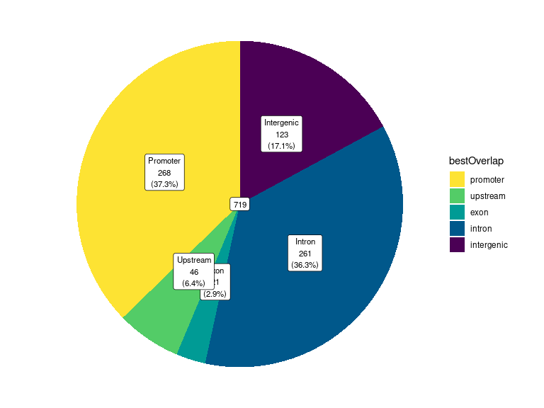
Pie chart showing customised labels. Here the regions have been modified to use title case in the labels, but without modifying the underlying data.
In addition to highly customisable labels, segments can be scaled by
width to produce segments representing the overlaps in kb instead of
counts, by setting scale_by = "width"
Split Donut Charts
Pie charts can be further extended into Split-Donut charts, with data in two rings. The default settings can be used to add the status of each window to the overlapping regions.
plotSplitDonut(
  tmm_results, inner = "bestOverlap", outer = "status",
  inner_palette = region_colours
)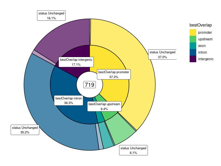
Split-Donut chart showing status with overlapping region
A key advantage of plotSplitDonut() is the ability to
provide separate colour palettes for the inner & outer rings. Once
again these are heavily customisable using the glue()
syntax for labels and exploding key segments of interest.
plotSplitDonut(
  tmm_results, inner = "bestOverlap", outer = "status",
  inner_palette = region_colours, outer_palette = status_colours,
  inner_glue = "{str_replace_all(.data[[inner]], ' ', '\n')}\nn = {comma(n)}\n{percent(p,0.1)}",
  outer_glue = "{.data[[outer]]}\n{str_replace_all(.data[[inner]], ' ', '\n')}\nn = {n}",
  explode_outer = "(In|De)creased", explode_r = 0.3,
  outer_label = "text", outer_min_p = 0, outer_max_p = 0.02
)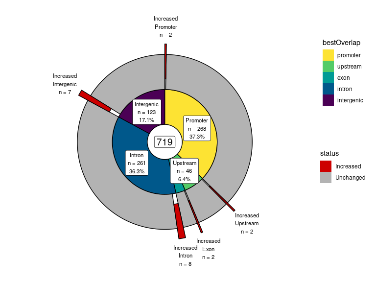
Split-Donut chart exploding key regions and customising labels.
Coverage Plots
In order to show our changed signal in context we can show the
coverage using a BigWigFileList and the function
plotHFGC(), which stands for plot HiC,
Features, Genes and
Coverage, with tracks appearing in that order.
plotHFGC() wraps multiple calls to the package
Gviz (Hahne and Ivanek 2016) to simplify repetitive plot
generation but retain significant flexibility. All tracks are options,
with the minimal requirements being cytogenetic bands along with a
specified GenomicRange. However, this does restrict plotting to the
“Standard Chromosomes”.
Coverage is produced using BigWig Files, passed to
plotHFGC() as either a BigWigFileList (for
separate tracks) or a list of BigWigFileList objects, for
multiple tracks with individual samples overlaid.
bwfl <- here::here(
  "data", "H3K27ac", glue("{levels(samples$treatment)}_cov_chr10.bw")
) %>%
  BigWigFileList() %>%
  setNames(levels(samples$treatment))
We can also include cytogenetic bands for these coverage plots, some
of which are provided with extraChIPs.
##   chrom chromStart chromEnd   name gieStain
## 1  chr1          0  2300000 p36.33     gneg
## 2  chr1    2300000  5400000 p36.32   gpos25
## 3  chr1    5400000  7200000 p36.31     gneg
## 4  chr1    7200000  9200000 p36.23   gpos25
## 5  chr1    9200000 12700000 p36.22     gneg
## 6  chr1   12700000 16200000 p36.21   gpos50
Let’s check the coverage across the most highly-ranked region with default settings.
gr <- filter(tmm_results, hmPValue_fdr < 0.05, str_detect(bestOverlap, '^Prom'))[1]The most important option to consider when showing coverage is whether to display tracks individually or as overlapping tracks. Passing a BigWigFileList will plot each file on a separate track by default, with y-axis limits able to be specified as consistent across all tracks. Alternatively, by passing the coverage as a list of BigWigFileList objects, each list element will be drawn as a single track with coverage overlaid. For one or more overlaid tracks, colours will need to now be provided in a list with matching structure.
The code for separate tracks would be: (not shown)
plotHFGC(gr, cytobands = grch37.cytobands, coverage = bwfl)Overlaying coverage onto a single track can instead be highly informative and enables the visualisation of multiple ChIP targets. (Plot not shown in vignette)
cov_list <- list(H3K27ac = bwfl)
cov_colour <- list(H3K27ac = treat_colours[levels(samples$treatment)])
plotHFGC(
  gr, cytobands = grch37.cytobands,
  coverage =  cov_list, linecol = cov_colour, zoom = 50, rotation.title = 90
)
By default, the specified range will also be outlined (i.e. highlighted) with a blue rectangle which is able to be turned off and customised as the user sees fit.
Adding Annotations To Coverage
An indication of which regions are associated with increased or
decreased ChIP signal can also be a useful annotation to add to plots
such as the above. Using the status from our differential signal
testing, we can create a GRangesList with the various
regions annotated as Increased, Unchanged etc,
Similar to the features track, where the names of
GRangesList elements denote the different feature types,
able to then assigned a colour, coverage annotation tracks follow these
same rules. For each coverage track being annotated, a
GRangesList object can denote the ranges which can be
assigned different colours. Annotation tracks should be passed to
plotHFGC() using the same structure as the coverage tracks,
so here if we pass the annotations as a list with the single element
H3K27ac these annotations will be added directly above the
coverage track for H3K27ac signal.
Displaying Genes and Features
Next we might like to add gene models to provide the regulatory
context. We’ll use the exons element of our gencode object
to create the format used by the defaults of the
GeneRegionTrack() function, with all exons and transcripts
annotated.
gene_models <- gencode$exon %>%
  select(
    type, gene = gene_id, exon = exon_id, transcript = transcript_id,
    symbol = gene_name
  )
Another useful track to add might be some key features such as
promoters and other annotated regions, as we have formed earlier in the
workflow. Features must always be a
GRangesList, with each element defining a different type of
feature, as we already have in our regions object. For
multiple feature tracks, a list of GRangesList objects can
be passed.
In our final plot, we’ll zoom out to the entire region covered by KAT6B, showing all transcripts, with out original region highlighted in blue. All merged windows for which a differential signal test was performed will be annotated with colours indicating the result for that window. As can be seen multiple H3K27ac signal regions appear to be responding to DHT treatment for KAT6B with a possible intronic enhancer and alternative promoter being most likely impacted, including the neighbouring region to our initial range. In contrast, the primary promoter appears unaffected by DHT treatment.
names(region_colours) <- names(regions)
plotHFGC(
  gr, cytobands = grch37.cytobands,
  features = regions, featcol = region_colours, featstack = "dense",
  coverage =  cov_list, linecol = cov_colour,
  genes = gene_models, genecol = "wheat", collapseTranscripts = FALSE,
  zoom = 350, shift = -1e5,
  rotation.title = 90, covsize = 10, genesize = 1, featsize = 5,
  annotation = cov_annot, annotcol = status_colours[c("Unchanged", "Increased")]
)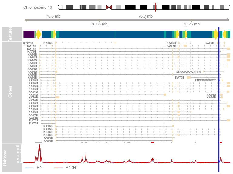
The addition of an annotation track for the coverage tracks shows which regions were retained during the analysis, as well as those which were considered as showing changed or unchanged signal
Plots are able to be tweaked considerably further via multiple
parameters, however these basic approaches cover the core functionality
of plotHFGC() for enabling simple & reproducible
plotting across regions for multiple sites within a larger
experiment.
If long-range interactions are available, these can also be provided as a GenomicInteractions object, completing all available options for the HFGC components.
Session Info
## R version 4.5.2 (2025-10-31)
## Platform: x86_64-pc-linux-gnu
## Running under: Ubuntu 24.04.3 LTS
##
## Matrix products: default
## BLAS:   /usr/lib/x86_64-linux-gnu/openblas-pthread/libblas.so.3
## LAPACK: /usr/lib/x86_64-linux-gnu/openblas-pthread/libopenblasp-r0.3.26.so;  LAPACK version 3.12.0
##
## locale:
##  [1] LC_CTYPE=en_US.UTF-8       LC_NUMERIC=C
##  [3] LC_TIME=en_US.UTF-8        LC_COLLATE=en_US.UTF-8
##  [5] LC_MONETARY=en_US.UTF-8    LC_MESSAGES=en_US.UTF-8
##  [7] LC_PAPER=en_US.UTF-8       LC_NAME=C
##  [9] LC_ADDRESS=C               LC_TELEPHONE=C
## [11] LC_MEASUREMENT=en_US.UTF-8 LC_IDENTIFICATION=C
##
## time zone: UTC
## tzcode source: system (glibc)
##
## attached base packages:
## [1] stats4    stats     graphics  grDevices utils     datasets  methods
## [8] base
##
## other attached packages:
##  [1] ggrepel_0.9.6               quantro_1.44.0
##  [3] magrittr_2.0.4              here_1.0.2
##  [5] glue_1.8.0                  scales_1.4.0
##  [7] plyranges_1.30.1            extraChIPs_1.14.2
##  [9] ggside_0.4.0                patchwork_1.3.2
## [11] edgeR_4.8.0                 limma_3.66.0
## [13] rtracklayer_1.70.0          BiocParallel_1.44.0
## [15] csaw_1.44.0                 SummarizedExperiment_1.40.0
## [17] Biobase_2.70.0              MatrixGenerics_1.22.0
## [19] matrixStats_1.5.0           Rsamtools_2.26.0
## [21] Biostrings_2.78.0           XVector_0.50.0
## [23] GenomicRanges_1.62.0        IRanges_2.44.0
## [25] S4Vectors_0.48.0            Seqinfo_1.0.0
## [27] BiocGenerics_0.56.0         generics_0.1.4
## [29] lubridate_1.9.4             forcats_1.0.1
## [31] stringr_1.6.0               dplyr_1.1.4
## [33] purrr_1.2.0                 readr_2.1.6
## [35] tidyr_1.3.1                 tibble_3.3.0
## [37] ggplot2_4.0.1               tidyverse_2.0.0
## [39] BiocStyle_2.38.0
##
## loaded via a namespace (and not attached):
##   [1] RColorBrewer_1.1-3        jsonlite_2.0.0
##   [3] GenomicFeatures_1.62.0    farver_2.1.2
##   [5] rmarkdown_2.30            fs_1.6.6
##   [7] BiocIO_1.20.0             ragg_1.5.0
##   [9] vctrs_0.6.5               multtest_2.66.0
##  [11] memoise_2.0.1             DelayedMatrixStats_1.32.0
##  [13] RCurl_1.98-1.17           askpass_1.2.1
##  [15] htmltools_0.5.8.1         S4Arrays_1.10.0
##  [17] curl_7.0.0                Rhdf5lib_1.32.0
##  [19] SparseArray_1.10.1        rhdf5_2.54.0
##  [21] sass_0.4.10               nor1mix_1.3-3
##  [23] bslib_0.9.0               htmlwidgets_1.6.4
##  [25] desc_1.4.3                plyr_1.8.9
##  [27] cachem_1.1.0              GenomicAlignments_1.46.0
##  [29] lifecycle_1.0.4           iterators_1.0.14
##  [31] pkgconfig_2.0.3           Matrix_1.7-4
##  [33] R6_2.6.1                  fastmap_1.2.0
##  [35] digest_0.6.38             siggenes_1.84.0
##  [37] reshape_0.8.10            AnnotationDbi_1.72.0
##  [39] rprojroot_2.1.1           RSQLite_2.4.4
##  [41] textshaping_1.0.4         base64_2.0.2
##  [43] timechange_0.3.0          httr_1.4.7
##  [45] abind_1.4-8               compiler_4.5.2
##  [47] beanplot_1.3.1            rngtools_1.5.2
##  [49] bit64_4.6.0-1             withr_3.0.2
##  [51] doParallel_1.0.17         S7_0.2.1
##  [53] DBI_1.2.3                 HDF5Array_1.38.0
##  [55] MASS_7.3-65               openssl_2.3.4
##  [57] DelayedArray_0.36.0       rjson_0.2.23
##  [59] tools_4.5.2               rentrez_1.2.4
##  [61] quadprog_1.5-8            h5mread_1.2.0
##  [63] restfulr_0.0.16           InteractionSet_1.38.0
##  [65] nlme_3.1-168              rhdf5filters_1.22.0
##  [67] grid_4.5.2                gtable_0.3.6
##  [69] tzdb_0.5.0                preprocessCore_1.72.0
##  [71] data.table_1.17.8         hms_1.1.4
##  [73] xml2_1.4.1                metapod_1.18.0
##  [75] foreach_1.5.2             pillar_1.11.1
##  [77] genefilter_1.92.0         splines_4.5.2
##  [79] lattice_0.22-7            bit_4.6.0
##  [81] survival_3.8-3            GEOquery_2.78.0
##  [83] annotate_1.88.0           tidyselect_1.2.1
##  [85] locfit_1.5-9.12           knitr_1.50
##  [87] bookdown_0.45             xfun_0.54
##  [89] scrime_1.3.5              statmod_1.5.1
##  [91] stringi_1.8.7             UCSC.utils_1.6.0
##  [93] yaml_2.3.10               evaluate_1.0.5
##  [95] codetools_0.2-20          cigarillo_1.0.0
##  [97] minfi_1.56.0              BiocManager_1.30.27
##  [99] cli_3.6.5                 bumphunter_1.52.0
## [101] xtable_1.8-4              systemfonts_1.3.1
## [103] jquerylib_0.1.4           dichromat_2.0-0.1
## [105] Rcpp_1.1.0                GenomeInfoDb_1.46.0
## [107] png_0.1-8                 XML_3.99-0.20
## [109] parallel_4.5.2            blob_1.2.4
## [111] pkgdown_2.2.0.9000        mclust_6.1.2
## [113] doRNG_1.8.6.2             sparseMatrixStats_1.22.0
## [115] bitops_1.0-9              illuminaio_0.52.0
## [117] crayon_1.5.3              rlang_1.1.6
## [119] KEGGREST_1.50.0