extraChIPs: Differential Signal Using Fixed-Width Windows
Stevie Pederson
Black Ochre Data Laboratories, Telethon Kids Institute, Adelaide, AustraliaJohn Curtin School of Medical Research, Australian National Universitystephen.pederson.au@gmail.com Source:
vignettes/differential_signal_fixed.Rmd
differential_signal_fixed.Rmd
knitr::opts_chunk$set(message = FALSE, crop = NULL)Introduction
The GRAVI workflow, for
which this package is designed, uses sliding windows for differential
signal analysis. However, the use of fixed-width windows, as is common
under DiffBind-style (Ross-Innes et al. 2012) approaches is also
possible with extraChIPs. This vignette focusses on using
conventional peak calls and fixed-width approaches to replicate and
extend these approaches.
The majority of examples below use heavily reduced datasets to provide general guidance on using the functions. Some results may appear trivial as a result, but will hopefully prove far more useful in a true experimental context. All data, along with this vignette are available here. Please place all contents of the data directory in a directory named data in your own working directory.
Setup
Installation
In order to use the package extraChIPs and follow this
vignette, we recommend using the package BiocManager hosted
on CRAN. Once this is installed, the additional packages required for
this vignette (tidyverse, Rsamtools,
csaw, BiocParallel and
rtracklayer) can also be installed.
if (!"BiocManager" %in% rownames(installed.packages()))
  install.packages("BiocManager")
pkg <- c(
  "tidyverse", "Rsamtools", "csaw", "BiocParallel", "rtracklayer", "edgeR",
  "patchwork", "extraChIPs", "plyranges", "scales", "here", "quantro"
)
BiocManager::install(pkg, update = FALSE)
Once these packages are installed, we can load them easily
Data
All data for this vignette is expected to be in a sub-directory of the working directory named “data”, and all paths will be predicated on this. Please ensure you have all data in this location, obtained from here.
The data itself is ChIP-Seq data targeting the Estrogen Receptor
(ER), and is taken from the cell-line ZR-75-1 cell-line using data from
the BioProject , Pre-processing was performed using the prepareChIPs
workflow, written in snakemake (Mölder et al. 2021) and all code is
available at https://github.com/smped/PRJNA509779. ER binding was
assessed under Vehicle (E2) and DHT-stimulated (E2DHT) conditions. Using
GRCh37 as the reference genome, a subset of regions found on chromosome
10 are included in this dataset for simplicity.
First we’ll define our sample data then define our two treatment groups. Defining a consistent colour palette for all plots is also a good habit to develop.
treat_levels <- c("E2", "E2DHT")
treat_colours <- setNames(c("steelblue", "red3"), treat_levels)
samples <- tibble(
  accession = paste0("SRR831518", seq(0, 5)),
  target = "ER",
  treatment = factor(rep(treat_levels, each = 3), levels = treat_levels)
)
samples
## # A tibble: 6 × 3
## accession target treatment
## <chr> <chr> <fct>
## 1 SRR8315180 ER E2
## 2 SRR8315181 ER E2
## 3 SRR8315182 ER E2
## 4 SRR8315183 ER E2DHT
## 5 SRR8315184 ER E2DHT
## 6 SRR8315185 ER E2DHTWe’ll eventually be loading counts for differential signal analysis
from a set of BamFiles, so first we’ll create a BamFileList
with all of these files.
bfl <- here("data", "ER", glue("{samples$accession}.bam")) %>%
  BamFileList() %>%
  setNames(str_remove_all(names(.), ".bam"))
file.exists(path(bfl))
## [1] TRUE TRUE TRUE TRUE TRUE TRUESeqinfo objects are the foundation of working with
GRanges, so defining an object at the start of a workflow is good
practice. This is simply enabled with extraChIPs by using
defineSeqinfo() and specifying the appropriate genome.
sq <- defineSeqinfo("GRCh37")Another key preparatory step for working with peaks is to define a set of regions as either blacklisted or grey-listed regions. The former are known problematic regions based on each genome, with data freely available from https://github.com/Boyle-Lab/Blacklist/tree/master/lists, whilst grey-listed regions are defined from potentially problematic regions as detected within the input sample. For our samples code for this is included in the previously provided repository (https://github.com/smped/PRJNA509779).
greylist <- import.bed(here("data/chr10_greylist.bed"), seqinfo = sq)
blacklist <- import.bed( here("data/chr10_blacklist.bed"), seqinfo = sq)
omit_ranges <- c(greylist, blacklist)
Working With Peaks
The provided dataset includes six files produced by
macs2 callpeak (Zhang et al. 2008) in the
narrowPeak format, and these are able to be easily parsed
using extraChIPs. We’ll immediately pass our black &
grey-listed regions to our parsing function so we can exclude these
regions right from the start. By passing the above seqinfo object to
this function, we’re also telling importPeaks() to ignore
any peaks not on the included chromosomes.
peaks <- here("data", "ER", glue("{samples$accession}_peaks.narrowPeak")) %>%
  importPeaks(seqinfo = sq, blacklist = omit_ranges)
This will import the peaks from all files as a single
GRangesList object, adding the file-name to each element by
default. We can easily modify these names if we so wish.
names(peaks) <- str_remove_all(names(peaks), "_peaks.narrowPeak")Once loaded, we can easily check how similar our replicates are using
plotOverlaps(). When three or more sets of peaks are
contained in the GRangesList, an UpSet plot will be drawn
by default.
plotOverlaps(
  peaks, min_size = 10, sort_sets = NULL,
  set_col = treat_colours[as.character(samples$treatment)]
)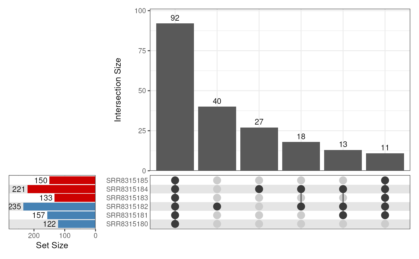
UpSet plot showing overlapping peaks across all replicates
Optionally, specifying a column and a suitable function will produce an additional panel summarising that value. In the following, we’ll show the maximum score obtained, highlighting that for peaks identified in only one or two replicates, the overall signal intensity is generally lower, even in the sample with the strongest signal.
plotOverlaps(
  peaks, min_size = 10, sort_sets = NULL, var = "score", f = "max",
   set_col = treat_colours[as.character(samples$treatment)]
)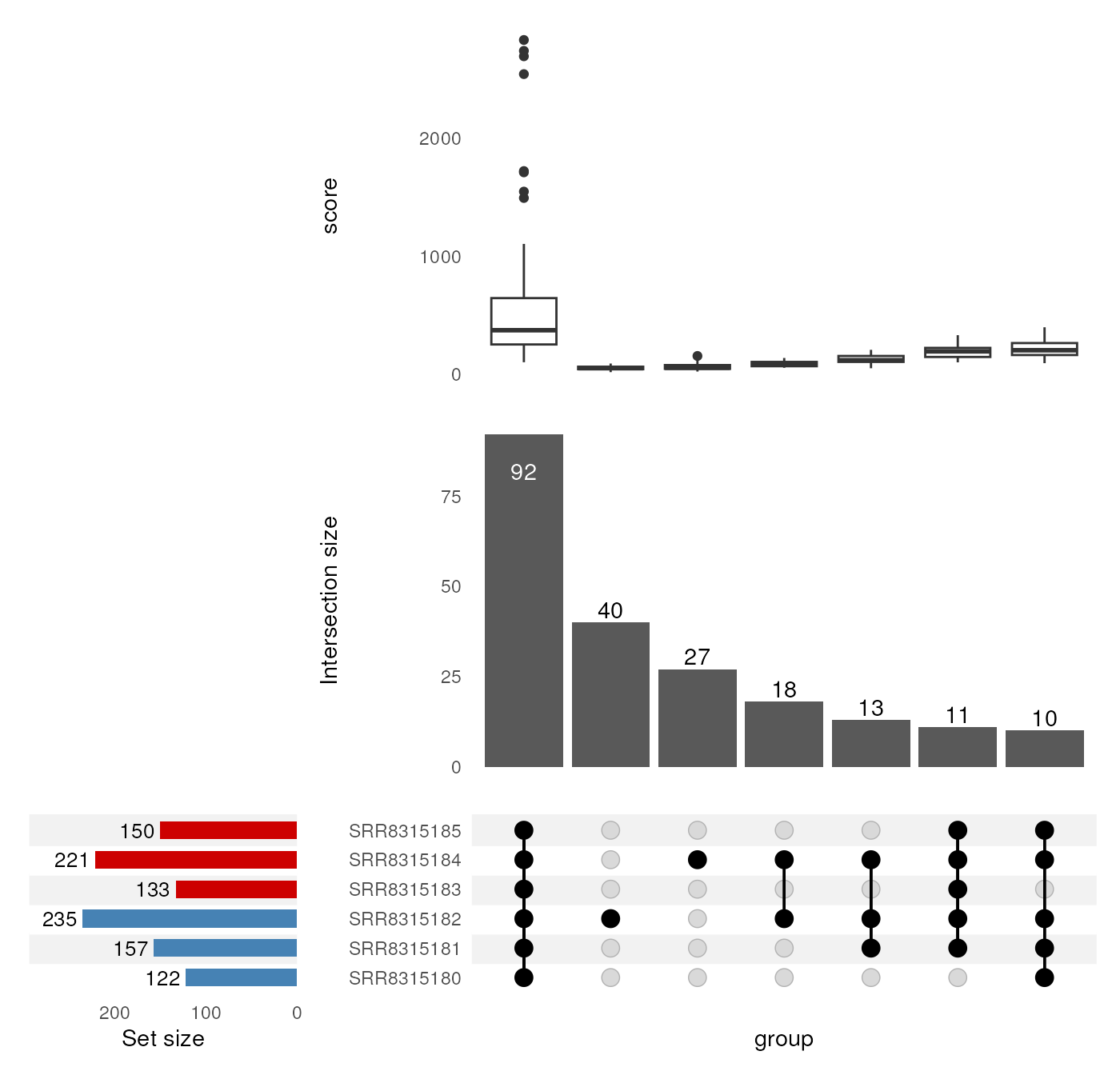
UpSet plot showing overlapping peaks across all replicates, with the maximum score across all replicates shown in the upper panel.
A common task at this point may be to define consensus peaks within
each treatment group, by retaining only the peaks found in 2 of the 3
replicates (p = 2/3). The default approach is to take the
union of all ranges, with the returned object containing logical values
for each sample, as well as the number of samples where an overlapping
peak was found.
If we wish to retain any of the original columns, such as the
macs2 callpeak score, we can simply pass the column names
to makeConsensus()
consensus_e2 <- makeConsensus(peaks[accessions$E2], p = 2/3, var = "score")
consensus_e2dht <- makeConsensus(peaks[accessions$E2DHT], p = 2/3, var = "score")
Alternatively, we could find the centre of the peaks as part of this process, by averaging across the estimated peak centres for each sample. This is a very common step for ChIP-Seq data where the target is a transcription factor, and also forms a key step in the DiffBind workflow.
In the following code chunk, we first find the centre for each sample
using the information provided by macs2, before retaining
this column when calling makeConsensus(). This will return
each of the individual centre-position estimates as a list for each
merged range, and using vapply() we then take the mean
position as our estimate for the combined peak centre.
consensus_e2 <- peaks[accessions$E2] %>%
  endoapply(mutate, centre = start + peak) %>%
  makeConsensus(p = 2/3, var = "centre") %>%
  mutate(centre = vapply(centre, mean, numeric(1)))
consensus_e2
## GRanges object with 164 ranges and 5 metadata columns:
## seqnames ranges strand | centre SRR8315180 SRR8315181
## <Rle> <IRanges> <Rle> | <numeric> <logical> <logical>
## [1] chr10 43048195-43048529 * | 43048362 TRUE TRUE
## [2] chr10 43521739-43522260 * | 43522020 TRUE TRUE
## [3] chr10 43540042-43540390 * | 43540272 TRUE FALSE
## [4] chr10 43606238-43606573 * | 43606416 TRUE TRUE
## [5] chr10 43851214-43851989 * | 43851719 FALSE TRUE
## ... ... ... ... . ... ... ...
## [160] chr10 99096784-99097428 * | 99097254 TRUE TRUE
## [161] chr10 99168353-99168649 * | 99168502 TRUE TRUE
## [162] chr10 99207868-99208156 * | 99207998 FALSE TRUE
## [163] chr10 99331363-99331730 * | 99331595 TRUE TRUE
## [164] chr10 99621632-99621961 * | 99621818 FALSE TRUE
## SRR8315182 n
## <logical> <numeric>
## [1] TRUE 3
## [2] TRUE 3
## [3] TRUE 2
## [4] TRUE 3
## [5] TRUE 2
## ... ... ...
## [160] TRUE 3
## [161] TRUE 3
## [162] TRUE 2
## [163] TRUE 3
## [164] TRUE 2
## -------
## seqinfo: 25 sequences from GRCh37 genome
consensus_e2dht <- peaks[accessions$E2DHT] %>%
  endoapply(mutate, centre = start + peak) %>%
  makeConsensus(p = 2/3, var = "centre") %>%
  mutate(centre = vapply(centre, mean, numeric(1)))
We can also inspect these using plotOverlaps() provided
we use a GRangesList for the input. Now that we only have
two elements (one for each treatment) a VennDiagram will be generated
instead of an UpSet plot.
GRangesList(E2 = granges(consensus_e2), E2DHT = granges(consensus_e2dht)) %>%
  plotOverlaps(set_col = treat_colours[treat_levels])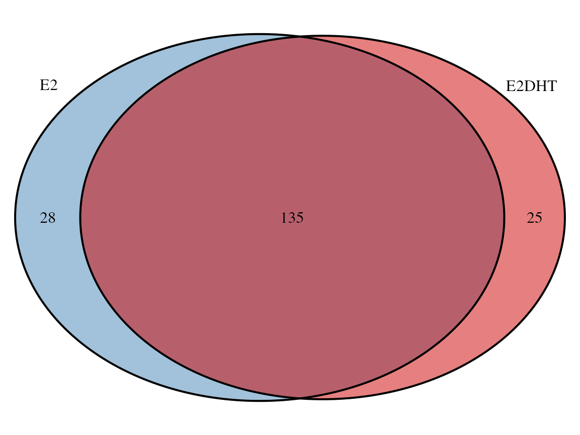
Overlap between consensus peaks identified in a treatment-specific manner
We can now go one step further and define the set of peaks found in either treatment. Given we’re being inclusive here, we can leave p = 0 so any peak found in either treatment is included.
union_peaks <- GRangesList(
  E2 = select(consensus_e2, centre),
  E2DHT = select(consensus_e2dht, centre)
) %>%
  makeConsensus(var = c("centre")) %>%
  mutate(
    centre = vapply(centre, mean, numeric(1)) %>% round(0)
  )
Now we have a set of peaks, found in at least 2/3 of samples from either condition, with estimates of each peak’s centre. The next step would be to set all peaks as the same width based on the centre position, with a common width being 500bp.
In the following we’ll perform multiple operations in a single call mutate, so let’s make sure we know what’s happening.
-
glue("{seqnames}:{centre}:{strand}")usesgluesyntax to parse the seqnames, centre position and strand information as a character-like vector with a width of only 1, and using the estimated centre as the Range. - We then coerce this to a
GRangesobject, before resizing to the desired width. - We also add the original (un-centred) range as an additional column,
retaining the
GRangesstructure, but discarding anything in themcols()element, then - Using
colToRanges(), we take the centred ranges and place them as the core set of GRanges for this object.
This gives a GRanges object with all original information, but with centred peaks of a fixed width.
Counting Reads
Now we have our centred, fixed-width peaks, we can count reads using
csaw::regionCounts() (Lun and Smyth 2016). We know our
fragment length is about 200bp, so we can pass this to the function for
a slightly more sophisticated approach to counting.
se <- regionCounts(bfl, centred_peaks, ext = 200)
se## class: RangedSummarizedExperiment
## dim: 188 6
## metadata(2): final.ext param
## assays(1): counts
## rownames: NULL
## rowData names(4): E2 E2DHT n union_peak
## colnames(6): SRR8315180 SRR8315181 ... SRR8315184 SRR8315185
## colData names(4): bam.files totals ext rlenThe colData() element of the returned object as the
columns bam.files, totals, ext and
rlen, which are all informative and can be supplemented with
our samples data frame. In the following, we’ll 1) coerce
to a tibble, 2) left_join() the
samples object, 3) add the accession as the sample column,
4) set the accession back as the rownames, then 5) coerce back to the
required DataFrame() structure.
colData(se) <- colData(se) %>%
  as_tibble(rownames = "accession") %>%
  left_join(samples) %>%
  mutate(sample = accession) %>%
  as.data.frame() %>%
  DataFrame(row.names = .$accession)
colData(se)
## DataFrame with 6 rows and 8 columns
## accession bam.files totals ext rlen
## <character> <character> <integer> <integer> <integer>
## SRR8315180 SRR8315180 /home/steviep/github.. 317845 200 75
## SRR8315181 SRR8315181 /home/steviep/github.. 337623 200 75
## SRR8315182 SRR8315182 /home/steviep/github.. 341998 200 75
## SRR8315183 SRR8315183 /home/steviep/github.. 315872 200 75
## SRR8315184 SRR8315184 /home/steviep/github.. 352908 200 75
## SRR8315185 SRR8315185 /home/steviep/github.. 347709 200 75
## target treatment sample
## <character> <factor> <character>
## SRR8315180 ER E2 SRR8315180
## SRR8315181 ER E2 SRR8315181
## SRR8315182 ER E2 SRR8315182
## SRR8315183 ER E2DHT SRR8315183
## SRR8315184 ER E2DHT SRR8315184
## SRR8315185 ER E2DHT SRR8315185For QC and visualisation, we can add an additional
logCPM assay to our object as well.
First we might like to check our distribution of counts
plotAssayDensities(se, assay = "counts", colour = "treat", trans = "log1p") +
  scale_colour_manual(values = treat_colours)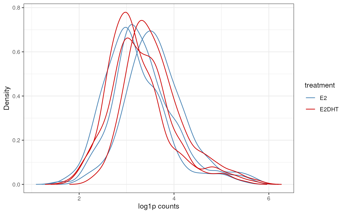
Count densities for all samples, using the log+1 transformation
A PCA plot can also provide insight as to where the variability in the data lies.
plotAssayPCA(se, assay = "logCPM", colour = "treat", label = "sample") +
  scale_colour_manual(values = treat_colours)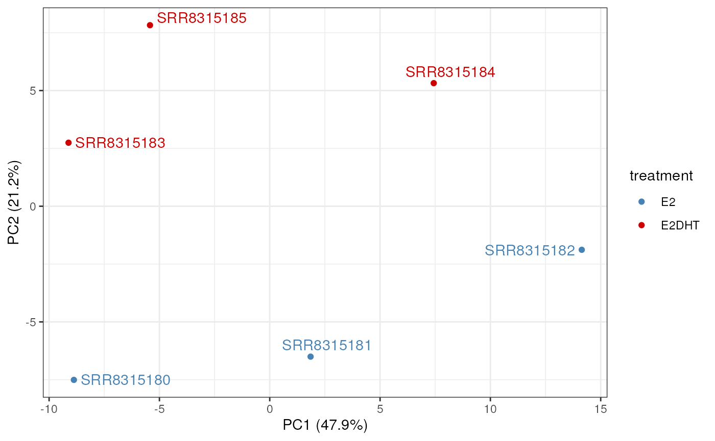
PCA plot using logCPM values and showing that replicate variability is larger than variability between treatment groups.
Differential Signal Analysis
Statistical Testing
In order to perform Differential Signal Analysis, we simply need to
define a model matrix, as for conventional analysis using
edgeR or limma. We can then pass this, along
with our fixed-width counts to fitAssayDiff(). By default
normalisation will be library-size normalisation, as is a
common default strategy for ChIP-Seq data. In contrast to sliding window
approaches, these results represent our final results and there is no
need for merging windows.
X <- model.matrix(~treatment, data = colData(se))
ls_res <- fitAssayDiff(se, design = X, asRanges = TRUE)
sum(ls_res$FDR < 0.05)
## [1] 2TMM normalisation (Robinson and Oshlack 2010) is another common
strategy, which relies on the data from all treatment groups being drawn
from the same distributions. We can formally test this using the package
quantro (Hicks and Irizarry 2015) , which produces p-values
for 1) H0: Group medians are drawn from the same
distribution, and 2) H0: Group-specific distributions are the
same.
## quantro: Test for global differences in distributions
##    nGroups:  2
##    nTotSamples:  6
##    nSamplesinGroups:  3 3
##    anovaPval:  0.90754
##    quantroStat:  0.21859
##    quantroPvalPerm:  0.572
Here, both p-values are >0.05, so in conjunction with out visual
inspection earlier, we can confidently apply TMM normalisation. To apply
this, we simply specify the argument norm = "TMM" when we
call fitAssayDiff(). In the analysis below, we’ve also
specified a fold-change threshold (fc = 1.2), below which,
changes in signal are considered to not be of interest (McCarthy and
Smyth 2009). This threshold is incorporated into the testing so there is
no requirement for post-hoc filtering based on a threshold.
tmm_res <- fitAssayDiff(se, design = X, norm = "TMM", asRanges = TRUE, fc = 1.2)
sum(tmm_res$FDR < 0.05)
## [1] 6An MA-plot is a common way of inspecting results and in the following we use the original ‘union_peak’ in our labelling of points. This serves as a reminder that the fixed-width windows are in fact a proxy for the entire region for which we have confidently detected ChIP signal, and that these windows are truly the regions of interest.
tmm_res %>%
  as_tibble() %>%
  mutate(`FDR < 0.05` = FDR < 0.05) %>%
  ggplot(aes(logCPM, logFC)) +
  geom_point(aes(colour = `FDR < 0.05`)) +
  geom_smooth(se = FALSE) +
  geom_label_repel(
    aes(label = union_peak), colour = "red",
    data = . %>% dplyr::filter(FDR < 0.05)
  ) +
  scale_colour_manual(values = c("black", "red"))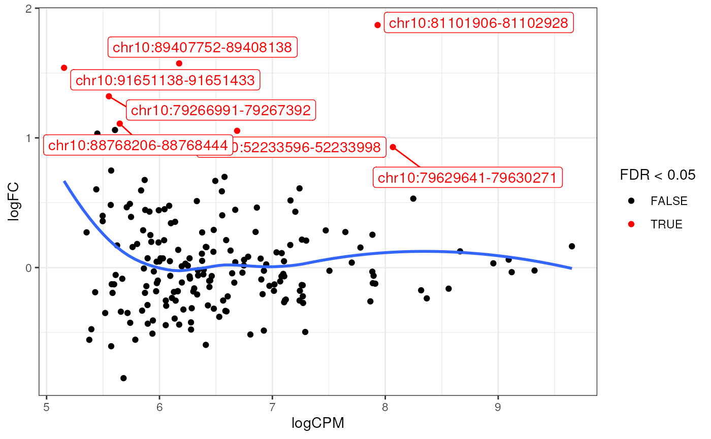
MA-plot after fitting using TMM normalisation and applying a fold-change threshold during testing. Points are labelled using the original windows obtained when merging replicates and treatment groups.
Mapping to Genes
Whilst knowledge of which regions are showing differential signal, the fundamental question we are usually asking is about the downstream regulatory consequences, such as the target gene. Before we can map peaks to genes, we’ll need to define our genes. In the following, we’ll use the provided Gencode gene mappings at the gene, transcript and exon level.
gencode <- here("data/gencode.v43lift37.chr10.annotation.gtf.gz") %>%
  import.gff() %>%
  filter_by_overlaps(GRanges("chr10:42354900-100000000")) %>%
  split(.$type)
seqlevels(gencode) <- seqlevels(sq)
seqinfo(gencode) <- sq
Mapping to genes using mapByFeature() uses additional
annotations, such as whether the peak overlaps a promoter, enhancer or
long-range interaction. Here we’ll just use promoters, so let’s create a
set of promoters from our transcript-level information, ensuring we
incorporate all possible promoters within a gene, and merging any
overlapping ranges using reduceMC()
promoters <- gencode$transcript %>%
    select(gene_id, ends_with("name")) %>%
    promoters(upstream = 2500, downstream = 500) %>%
    reduceMC(simplify = FALSE)
promoters
## GRanges object with 1678 ranges and 3 metadata columns:
## seqnames ranges strand |
## <Rle> <IRanges> <Rle> |
## [1] chr10 42678287-42681286 + |
## [2] chr10 42702938-42705937 + |
## [3] chr10 42735669-42738668 + |
## [4] chr10 42743933-42746932 + |
## [5] chr10 42968428-42973155 + |
## ... ... ... ... .
## [1674] chr10 99635155-99638154 - |
## [1675] chr10 99643500-99646805 - |
## [1676] chr10 99695536-99698535 - |
## [1677] chr10 99770595-99773594 - |
## [1678] chr10 99789879-99793085 - |
## gene_id
## <CharacterList>
## [1] ENSG00000237592.2_5
## [2] ENSG00000271650.1_7
## [3] ENSG00000290458.1_2
## [4] ENSG00000274167.5_8
## [5] ENSG00000185904.12_9,ENSG00000185904.12_9,ENSG00000185904.12_9,...
## ... ...
## [1674] ENSG00000265398.1
## [1675] ENSG00000095713.14_13,ENSG00000095713.14_13
## [1676] ENSG00000095713.14_13
## [1677] ENSG00000095713.14_13
## [1678] ENSG00000095713.14_13,ENSG00000095713.14_13
## gene_name
## <CharacterList>
## [1] IGKV1OR10-1
## [2] ENSG00000271650
## [3] ENSG00000290458
## [4] ENSG00000274167
## [5] LINC00839,LINC00839,LINC00839,...
## ... ...
## [1674] AL139239.1
## [1675] CRTAC1,CRTAC1
## [1676] CRTAC1
## [1677] CRTAC1
## [1678] CRTAC1,CRTAC1
## transcript_name
## <CharacterList>
## [1] IGKV1OR10-1-201
## [2] ENST00000605702
## [3] ENST00000622823
## [4] ENST00000622650
## [5] LINC00839-204,LINC00839-203,LINC00839-202,...
## ... ...
## [1674] AL139239.1-201
## [1675] CRTAC1-205,CRTAC1-206
## [1676] CRTAC1-204
## [1677] CRTAC1-201
## [1678] CRTAC1-203,CRTAC1-202
## -------
## seqinfo: 25 sequences from GRCh37 genomeNow we’ll pass these to mapByFeature(), but first, we’ll
place the original ‘union_peak’ back as the core of the GRanges object.
This will retain all the results from testing, but ensures the correct
region is mapped to genes.
tmm_mapped_res <- tmm_res %>%
  colToRanges("union_peak") %>%
  mapByFeature(genes = gencode$gene, prom = promoters) %>%
  addDiffStatus()
arrange(tmm_mapped_res, PValue)
## GRanges object with 188 ranges and 11 metadata columns:
## seqnames ranges strand | E2 E2DHT n
## <Rle> <IRanges> <Rle> | <logical> <logical> <numeric>
## [1] chr10 81101906-81102928 * | TRUE TRUE 2
## [2] chr10 79629641-79630271 * | TRUE TRUE 2
## [3] chr10 89407752-89408138 * | FALSE TRUE 1
## [4] chr10 52233596-52233998 * | TRUE TRUE 2
## [5] chr10 91651138-91651433 * | FALSE TRUE 1
## ... ... ... ... . ... ... ...
## [184] chr10 57899195-57899649 * | TRUE TRUE 2
## [185] chr10 79190987-79191351 * | FALSE TRUE 1
## [186] chr10 93120411-93121224 * | TRUE TRUE 2
## [187] chr10 84812327-84812615 * | TRUE FALSE 1
## [188] chr10 95755308-95755721 * | TRUE TRUE 2
## logFC logCPM PValue FDR p_mu0
## <numeric> <numeric> <numeric> <numeric> <numeric>
## [1] 1.871060 7.93229 3.32981e-24 6.26004e-22 5.86555e-30
## [2] 0.931608 8.06748 1.77568e-07 1.66914e-05 7.16573e-11
## [3] 1.570273 6.17416 6.05081e-07 3.79184e-05 6.73569e-08
## [4] 1.049765 6.68775 5.82639e-05 2.73840e-03 5.28527e-06
## [5] 1.539043 5.15469 1.94038e-04 7.29583e-03 6.91838e-05
## ... ... ... ... ... ...
## [184] 0.01656860 6.74759 0.949645 0.970289 0.939137
## [185] -0.01280716 6.39247 0.963207 0.972684 0.958637
## [186] -0.02142115 9.32215 0.963659 0.972684 0.831820
## [187] 0.01237140 6.19732 0.967510 0.972684 0.963156
## [188] -0.00530365 5.86168 0.986505 0.986505 0.985630
## gene_id
## <CharacterList>
## [1] ENSG00000108179.14_6
## [2] ENSG00000151208.17_11
## [3] ENSG00000225913.2_9,ENSG00000196566.2_10
## [4] ENSG00000198964.14_10,ENSG00000225303.2_10
## [5] ENSG00000280560.3_9
## ... ...
## [184]
## [185] ENSG00000156113.25_17
## [186] ENSG00000289228.2_2
## [187] ENSG00000200774.1
## [188] ENSG00000138193.17_12
## gene_name status
## <CharacterList> <factor>
## [1] PPIF Increased
## [2] DLG5 Increased
## [3] ENSG00000225913,ENSG00000196566 Increased
## [4] SGMS1,ENSG00000225303 Increased
## [5] LINC01374 Increased
## ... ... ...
## [184] Unchanged
## [185] KCNMA1 Unchanged
## [186] ENSG00000289228 Unchanged
## [187] RNU6-478P Unchanged
## [188] PLCE1 Unchanged
## -------
## seqinfo: 24 sequences from GRCh37 genomeInspection of Results
Profile Heatmaps
When analysing a transcription factor, checking the binding profile across our treatment groups can be informative, and is often performed using ‘Profile Heatmaps’ where coverage is smoothed within bins surrounding our peak centre.
The function getProfileData() takes a set of ranges and
a BigWigFileList, and performs the smoothing, which is then passed to
the function plotProfileHeatmap().
The following shows the three steps of 1) defining the ranges, 2) obtaining the smoothed binding profiles, and 3) drawing the heatmap. Note that we can facet the heatmaps by selecting the ‘status’ column to separate any Increased or Decreased regions. By default, this will also draw the smoothed lines in the top panel using different colours.
These plots can be used to show coverage-like values (SPMR or CPM) or
we can use fold-enrichment over the input sample(s), as is also produced
by macs2 bdgcmp. This data isn’t generally visualised using
log-transformation so we’ll set log = FALSE in our call to
getProfileData()
fe_bw <- here("data", "ER", glue("{treat_levels}_FE_chr10.bw")) %>%
  BigWigFileList() %>%
  setNames(treat_levels)
sig_ranges <- filter(tmm_mapped_res, FDR < 0.05)
pd_fe <- getProfileData(fe_bw, sig_ranges, log = FALSE)
pd_fe %>%
  plotProfileHeatmap("profile_data", facetY = "status") +
  scale_fill_gradient(low = "white", high = "red") +
  labs(fill = "Fold\nEnrichment")
Session Info
## R version 4.5.2 (2025-10-31)
## Platform: x86_64-pc-linux-gnu
## Running under: Ubuntu 24.04.3 LTS
##
## Matrix products: default
## BLAS:   /usr/lib/x86_64-linux-gnu/openblas-pthread/libblas.so.3
## LAPACK: /usr/lib/x86_64-linux-gnu/openblas-pthread/libopenblasp-r0.3.26.so;  LAPACK version 3.12.0
##
## locale:
##  [1] LC_CTYPE=en_US.UTF-8       LC_NUMERIC=C
##  [3] LC_TIME=en_US.UTF-8        LC_COLLATE=en_US.UTF-8
##  [5] LC_MONETARY=en_US.UTF-8    LC_MESSAGES=en_US.UTF-8
##  [7] LC_PAPER=en_US.UTF-8       LC_NAME=C
##  [9] LC_ADDRESS=C               LC_TELEPHONE=C
## [11] LC_MEASUREMENT=en_US.UTF-8 LC_IDENTIFICATION=C
##
## time zone: UTC
## tzcode source: system (glibc)
##
## attached base packages:
## [1] stats4    stats     graphics  grDevices utils     datasets  methods
## [8] base
##
## other attached packages:
##  [1] quantro_1.44.0              here_1.0.2
##  [3] ggrepel_0.9.6               glue_1.8.0
##  [5] scales_1.4.0                plyranges_1.30.1
##  [7] extraChIPs_1.14.2           ggside_0.4.0
##  [9] patchwork_1.3.2             edgeR_4.8.0
## [11] limma_3.66.0                rtracklayer_1.70.0
## [13] BiocParallel_1.44.0         csaw_1.44.0
## [15] SummarizedExperiment_1.40.0 Biobase_2.70.0
## [17] MatrixGenerics_1.22.0       matrixStats_1.5.0
## [19] Rsamtools_2.26.0            Biostrings_2.78.0
## [21] XVector_0.50.0              GenomicRanges_1.62.0
## [23] IRanges_2.44.0              S4Vectors_0.48.0
## [25] Seqinfo_1.0.0               BiocGenerics_0.56.0
## [27] generics_0.1.4              lubridate_1.9.4
## [29] forcats_1.0.1               stringr_1.6.0
## [31] dplyr_1.1.4                 purrr_1.2.0
## [33] readr_2.1.6                 tidyr_1.3.1
## [35] tibble_3.3.0                ggplot2_4.0.1
## [37] tidyverse_2.0.0             BiocStyle_2.38.0
##
## loaded via a namespace (and not attached):
##   [1] splines_4.5.2             BiocIO_1.20.0
##   [3] bitops_1.0-9              preprocessCore_1.72.0
##   [5] XML_3.99-0.20             lifecycle_1.0.4
##   [7] doParallel_1.0.17         rprojroot_2.1.1
##   [9] lattice_0.22-7            MASS_7.3-65
##  [11] base64_2.0.2              scrime_1.3.5
##  [13] magrittr_2.0.4            minfi_1.56.0
##  [15] sass_0.4.10               rmarkdown_2.30
##  [17] jquerylib_0.1.4           yaml_2.3.10
##  [19] metapod_1.18.0            doRNG_1.8.6.2
##  [21] askpass_1.2.1             DBI_1.2.3
##  [23] RColorBrewer_1.1-3        abind_1.4-8
##  [25] quadprog_1.5-8            RCurl_1.98-1.17
##  [27] rentrez_1.2.4             genefilter_1.92.0
##  [29] SimpleUpset_0.1.3         annotate_1.88.0
##  [31] pkgdown_2.2.0.9000        DelayedMatrixStats_1.32.0
##  [33] codetools_0.2-20          DelayedArray_0.36.0
##  [35] xml2_1.4.1                tidyselect_1.2.1
##  [37] futile.logger_1.4.3       UCSC.utils_1.6.0
##  [39] farver_2.1.2              beanplot_1.3.1
##  [41] illuminaio_0.52.0         GenomicAlignments_1.46.0
##  [43] jsonlite_2.0.0            multtest_2.66.0
##  [45] survival_3.8-3            iterators_1.0.14
##  [47] systemfonts_1.3.1         foreach_1.5.2
##  [49] tools_4.5.2               ragg_1.5.0
##  [51] Rcpp_1.1.0                SparseArray_1.10.1
##  [53] mgcv_1.9-4                xfun_0.54
##  [55] GenomeInfoDb_1.46.0       HDF5Array_1.38.0
##  [57] withr_3.0.2               formatR_1.14
##  [59] BiocManager_1.30.27       fastmap_1.2.0
##  [61] rhdf5filters_1.22.0       openssl_2.3.4
##  [63] digest_0.6.38             timechange_0.3.0
##  [65] R6_2.6.1                  textshaping_1.0.4
##  [67] dichromat_2.0-0.1         RSQLite_2.4.4
##  [69] cigarillo_1.0.0           h5mread_1.2.0
##  [71] utf8_1.2.6                data.table_1.17.8
##  [73] InteractionSet_1.38.0     httr_1.4.7
##  [75] htmlwidgets_1.6.4         S4Arrays_1.10.0
##  [77] pkgconfig_2.0.3           gtable_0.3.6
##  [79] blob_1.2.4                S7_0.2.1
##  [81] siggenes_1.84.0           htmltools_0.5.8.1
##  [83] bookdown_0.45             png_0.1-8
##  [85] lambda.r_1.2.4            knitr_1.50
##  [87] tzdb_0.5.0                rjson_0.2.23
##  [89] nlme_3.1-168              curl_7.0.0
##  [91] bumphunter_1.52.0         cachem_1.1.0
##  [93] rhdf5_2.54.0              parallel_4.5.2
##  [95] AnnotationDbi_1.72.0      restfulr_0.0.16
##  [97] desc_1.4.3                GEOquery_2.78.0
##  [99] pillar_1.11.1             grid_4.5.2
## [101] reshape_0.8.10            vctrs_0.6.5
## [103] xtable_1.8-4              evaluate_1.0.5
## [105] VennDiagram_1.7.3         GenomicFeatures_1.62.0
## [107] futile.options_1.0.1      cli_3.6.5
## [109] locfit_1.5-9.12           compiler_4.5.2
## [111] rlang_1.1.6               crayon_1.5.3
## [113] rngtools_1.5.2            labeling_0.4.3
## [115] nor1mix_1.3-3             mclust_6.1.2
## [117] plyr_1.8.9                fs_1.6.6
## [119] stringi_1.8.7             Matrix_1.7-4
## [121] hms_1.1.4                 sparseMatrixStats_1.22.0
## [123] bit64_4.6.0-1             Rhdf5lib_1.32.0
## [125] KEGGREST_1.50.0           statmod_1.5.1
## [127] memoise_2.0.1             bslib_0.9.0
## [129] bit_4.6.0