Draw a coverage Profile Heatmap

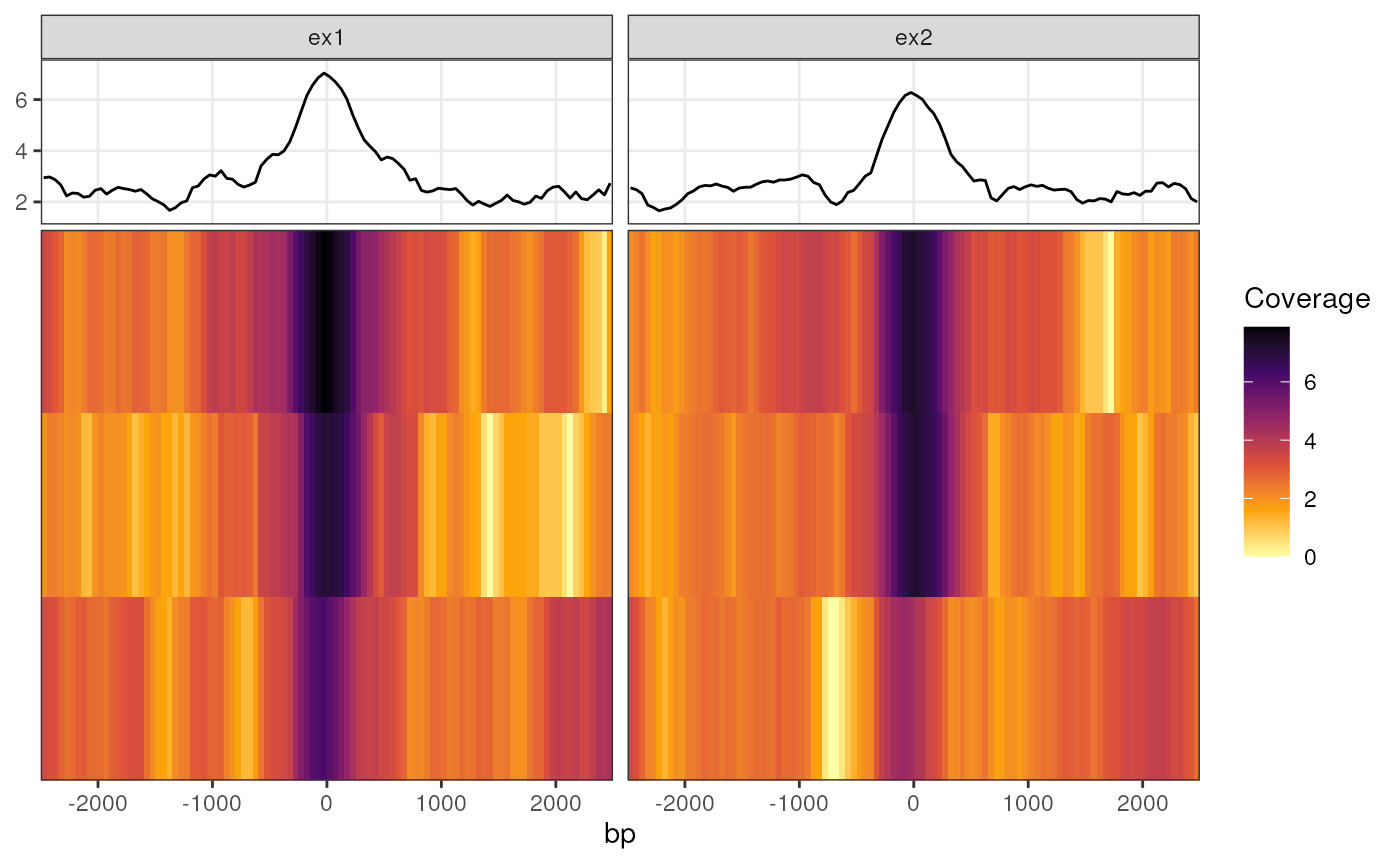
Plot a coverage Profile Heatmap across multiple ranges

plotProfileHeatmap(object, ...)

# S4 method for class 'GenomicRangesList'
plotProfileHeatmap(
  object,
  profileCol = "profile_data",
  xValue = "bp",
  fillValue = "score",
  facetX = NULL,
  facetY = NULL,
  colour = facetY,
  linetype = NULL,
  summariseBy = c("mean", "median", "min", "max", "none"),
  xLab = xValue,
  yLab = NULL,
  fillLab = fillValue,
  labelFunX = waiver(),
  relHeight = 0.3,
  sortFilter = NULL,
  maxDist = 100,
  ...
)

# S4 method for class 'GenomicRanges'
plotProfileHeatmap(
  object,
  profileCol = "profile_data",
  xValue = "bp",
  fillValue = "score",
  facetX = NULL,
  facetY = NULL,
  colour = facetY,
  linetype = NULL,
  summariseBy = c("mean", "median", "min", "max", "none"),
  xLab = xValue,
  yLab = NULL,
  fillLab = fillValue,
  labelFunX = waiver(),
  relHeight = 0.3,
  summaryLabelSide = "left",
  respectLevels = FALSE,
  sortFilter = NULL,
  maxDist = 100,
  ...
)

Arguments

object

A GRanges or GRangesList object

...

Passed to facet_grid internally. Can be utilised for switching panel strips or passing a labeller function

profileCol

Column name specifying where to find the profile DataFrames

xValue, fillValue

Columns within the profile DataFrames for heatmaps

facetX, facetY

Columns used for faceting across the x- or y-axis respectively

colour

Column used for colouring lines in the summary panel. Defaults to any column used for facetY

linetype

Column used for linetypes in the summary panel

summariseBy

Function for creating the summary plot in the top panel. If set to 'none', no summary plot will be drawn. Otherwise the top panel will contain a line-plot representing this summary value for each x-axis bin

xLab, yLab, fillLab

Labels for plotting aesthetics. Can be overwritten using labs() on any returned object

labelFunX

Function for formatting x-axis labels

relHeight

The relative height of the top summary panel. Represents the fraction of the plotting area taken up by the summary panel.

sortFilter

If calling on a GRangesList, a method for subsetting the original object (e.g. 1:2). If calling on a GRanges object should be and expression able to be parsed as a filtering expression using eval_tidy. This is applied when sorting the range order down the heatmap such that ranges can be sorted by one or specific samples, or all. Ranges will always be sorted such that those with the strongest signal are at the top of the plot

maxDist

Maximum distance from the centre to find the strongest signal when arranging the ranges

summaryLabelSide

Side to place y-axis for the summary plot in the top panel

respectLevels

logical(1) If FALSE, facets along the y-axis will be arranged in descending order of signal, otherwise any original factor levels will be retained

Value

A ggplot2 object, able to be customised using standard ggplot2 syntax

Details

Convenience function for plotting coverage heatmaps across a common set of ranges, shared between one or more samples. These are most commonly the coverage values from merged samples within a treatment group. THe input data structure is based on that obtained from getProfileData, and can be provided either as a GRanges object (generally for one sample) or as a GRangesList.

A 'profile DataFrame' here refers to a data.frame (or tibble, or DataFrame) with a coverage value in one column that corresponds to a genomic bin of a fixed size denoted in another, as generated by getProfileData. Given that multiple ranges are most likely to be drawn, each profile data frame must be the same size in terms of the number of bins, each of which represent a fixed number of nucleotides. At a minimum this is a two column data frame although getProfileData will provide three columns for each specified genomic region.

If using a GRangesList, each list element will be drawn as a separate panel by default. These panels will appear in the same order as the list elements of the GRangesList, although this can easily be overwritten by passing a column name to the facetX argument. The default approach will add the original element names as the column "name" which can be seen in the $data element of any resultant ggplot object produced by this function.

Examples

# \donttest{
library(rtracklayer)
fl <- system.file(
"extdata", "bigwig", c("ex1.bw", "ex2.bw"), package = "extraChIPs"
)
bwfl <- BigWigFileList(fl)
names(bwfl) <- c("ex1", "ex2")

gr <- GRanges(
  c(
    "chr10:103880281-103880460", "chr10:103892581-103892760",
    "chr10:103877281-103877460"
   )
)
pd <- getProfileData(bwfl, gr)
plotProfileHeatmap(pd, "profile_data") +
  scale_fill_viridis_c(option = "inferno", direction = -1) +
  labs(fill = "Coverage")

# }