QC: Raw Data
12 July, 2023
library(tidyverse)
library(glue)
library(yaml)
library(here)
library(reactable)
library(pander)
library(ngsReports)
library(scales)
library(htmltools)
library(Polychrome)
myTheme <- theme(
    plot.title = element_text(hjust = 0.5),
    text = element_text(size = 13)
  )
config <- read_yaml(here::here("config/config.yml"))
samples <- read_tsv(here::here(config$samples)) %>%
bind_rows(
tibble(
accession = unique(.$input), target = "Input"
)
)
n <- length(samples$accession)
pal <- createPalette(n, c("#2A95E8", "#E5629C"), range = c(10, 60), M = 100000)
names(pal) <- samples$accession
colours <- scale_colour_manual(values = pal)
qc_path <- here::here(config$paths$qc, "raw")
rel_qc_path <- ifelse(
grepl("docs", qc_path), gsub(".+docs", ".", qc_path),
gsub(here::here(), "..", qc_path)
)
fl <- file.path(qc_path, glue("{samples$accession}_fastqc.zip")) %>%
setNames(samples$accession)
rawFqc <- FastqcDataList(fl[file.exists(fl)])
names(rawFqc) <- names(fl)[file.exists(fl)]Introduction
This page provides summary statistics and diagnostics for the raw data as obtained at the commencement of the workflow. Most data was obtained from FastQC and parsed using the Bioconductor package ngsReports (Ward, To, and Pederson 2020). FastQC reports for 19 files were found.
A conventional MultiQC report (Ewels et al. 2016) can also be found here
Data Summary
div(
  class = "table",
  div(
    class = "table-header",
    htmltools::tags$caption(
      htmltools::em(
        "Library sizes with links to all raw FastQC reports"
      )
    )
  ),
  readTotals(rawFqc) %>%
    mutate(Filename = str_remove_all(Filename, ".(fast|f)q.gz")) %>%
    left_join(samples, by = c("Filename" = "accession")) %>%
    dplyr::select(-input) %>%
    setNames(str_replace_all(names(.), "_", " ")) %>%
    setNames(str_to_title(names(.))) %>%
    reactable(
      sortable = TRUE, resizable = TRUE,
      showPageSizeOptions = TRUE,
      columns = list(
        Filename = colDef(
          cell = function(value) htmltools::tags$a(
            href = file.path(rel_qc_path, glue("{value}_fastqc.html")),
            target = "_blank",
            value
          ),
          html = TRUE
        )
      ),
      defaultColDef = colDef(format = colFormat(separators = TRUE))
    )
)FastQC Status
plotSummary(rawFqc) + myTheme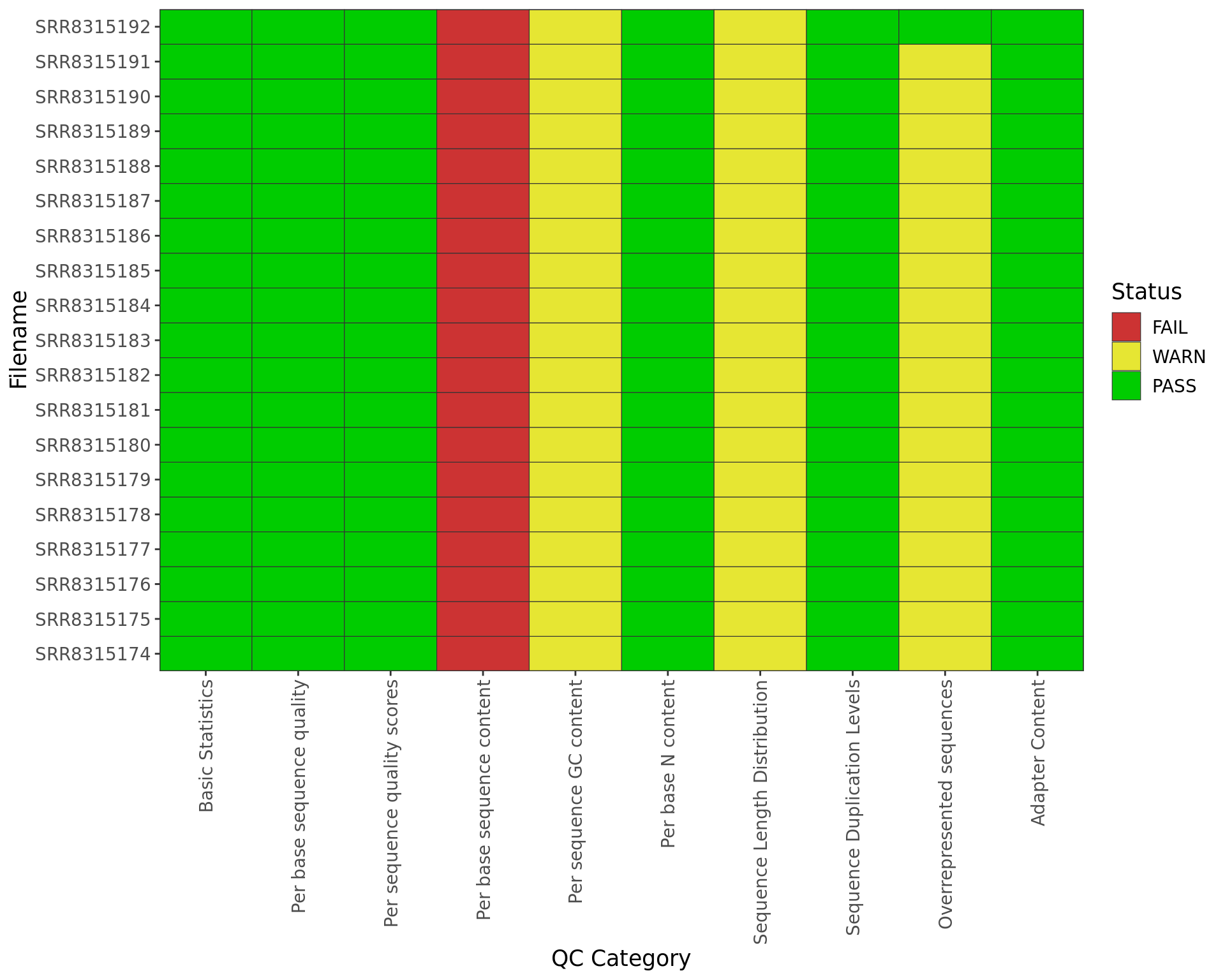
Summary of Pass/Warn/Fail status from all samples
Read Totals
p <- plotReadTotals(rawFqc, divBy = 1e6) + myTheme
p$data <- left_join(p$data, samples, by = c("Filename" = "accession"))
p + facet_grid(target + treatment ~ ., scales = "free", space = "free")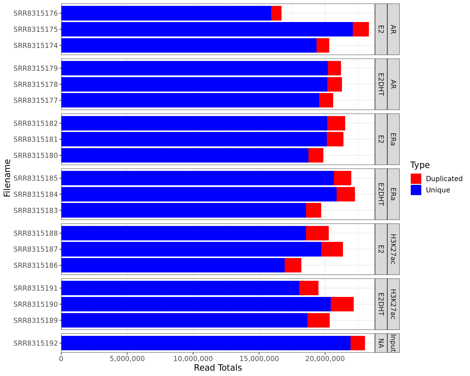
Raw library sizes showing estimated duplication levels
QC Diagnostics
Quality Scores
plotBaseQuals(rawFqc, heat_w = 20, dendrogram = TRUE, usePlotly = TRUE, text = element_text(size = 13))Mean Quality Scores are each position along the reads
Sequence Content Heatmap
plotSeqContent(rawFqc, usePlotly = TRUE, dendrogram = TRUE, heat_w = 20, text = element_text(size = 13))Sequence content along each read
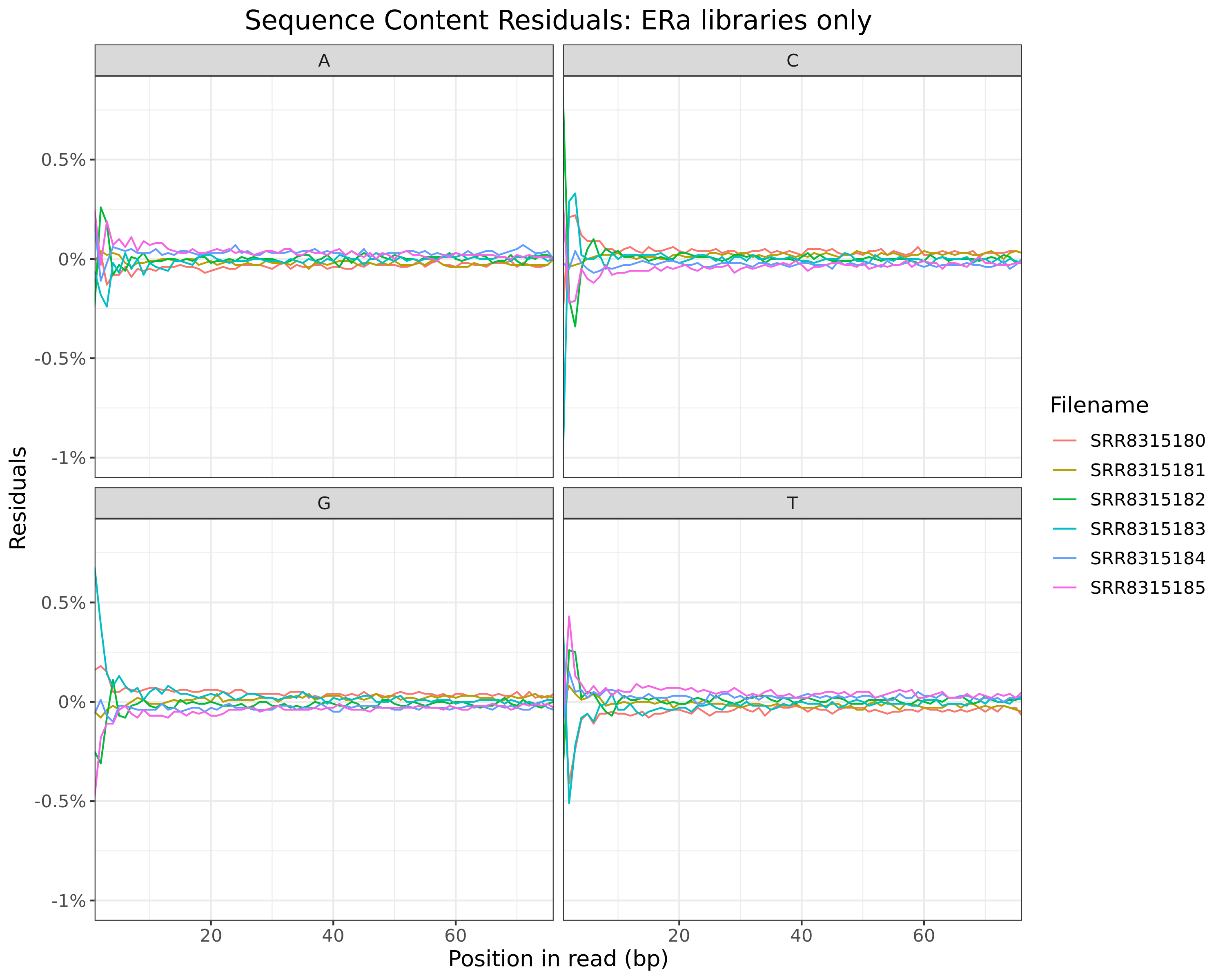
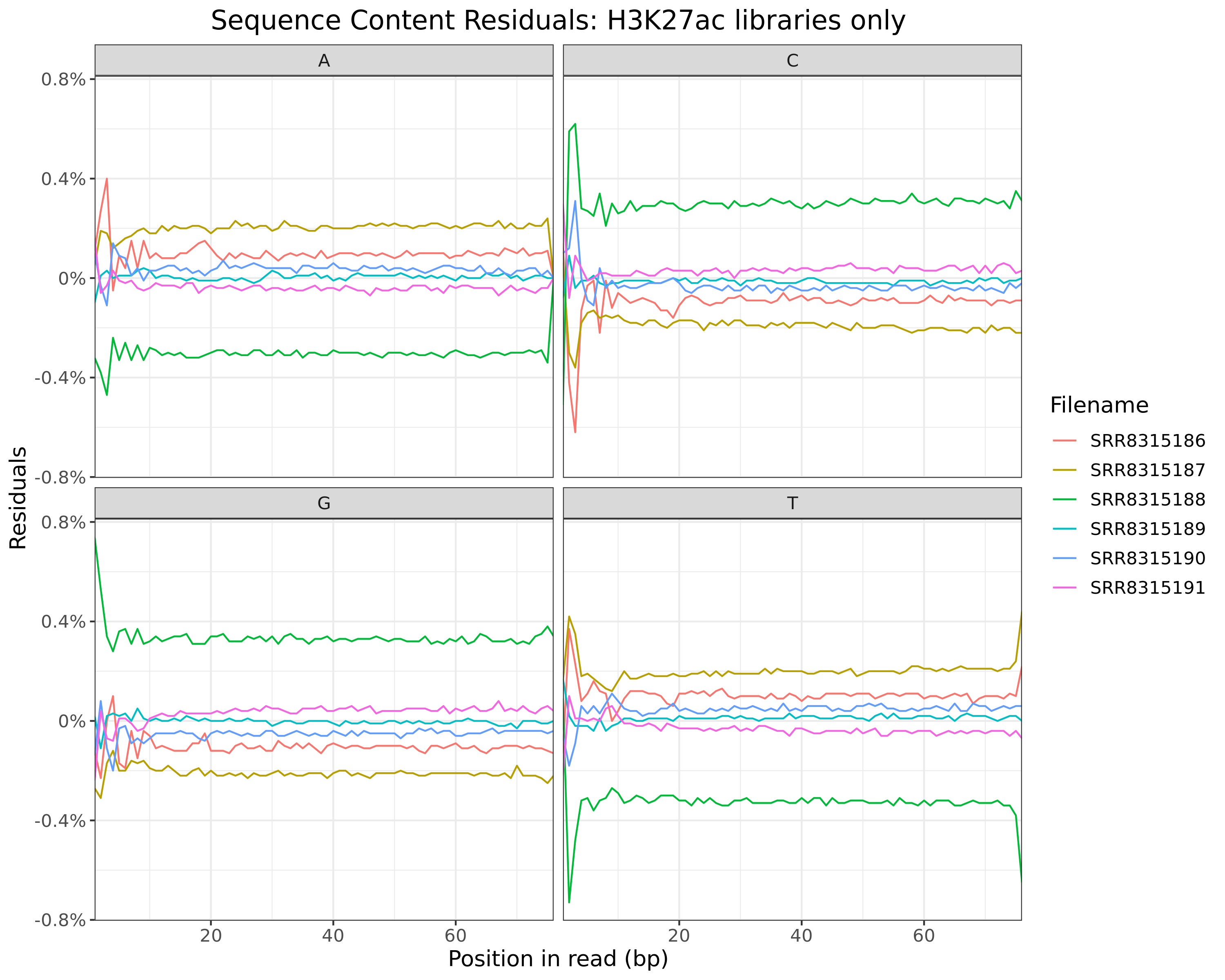
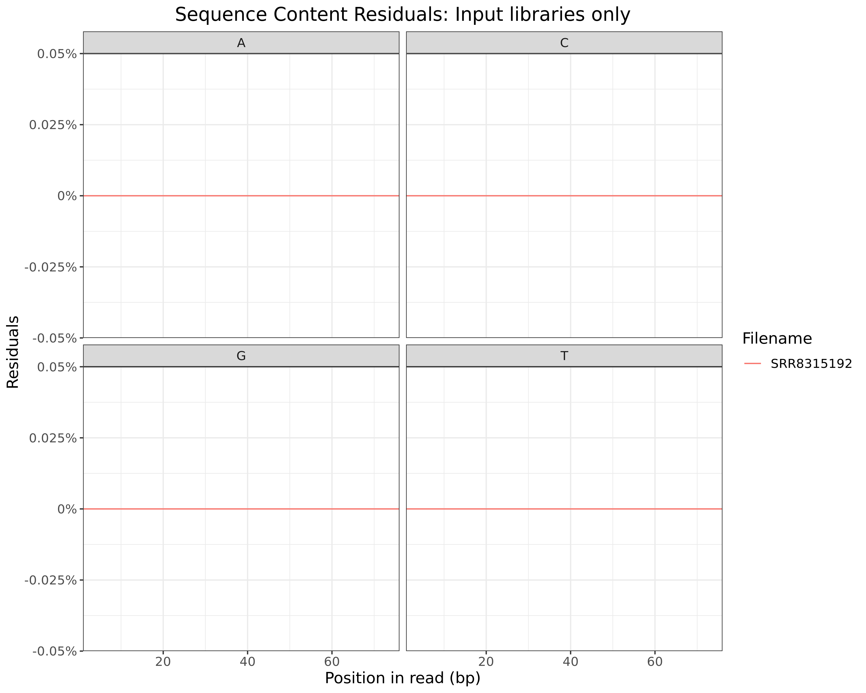
Sequence Content Residuals
All Libraries
plotSeqContent(rawFqc, plotType = "residuals", scaleColour = colours) + myTheme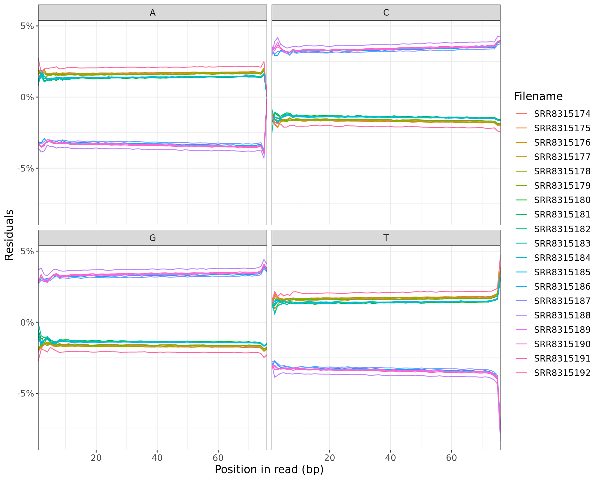
Residuals obtained when subtracting mean values at each position
d <- here::here("docs", "assets", "raw_fqc")
if (!dir.exists(d)) dir.create(d, recursive = TRUE)
h <- knitr::opts_chunk$get("fig.height")
w <- knitr::opts_chunk$get("fig.width")
htmltools::tagList(
samples %>%
dplyr::filter(accession %in% names(rawFqc)) %>%
split(.$target) %>%
setNames(NULL) %>%
lapply(
function(x) {
tgt <- unique(x$target)
fqc <- rawFqc[x$accession]
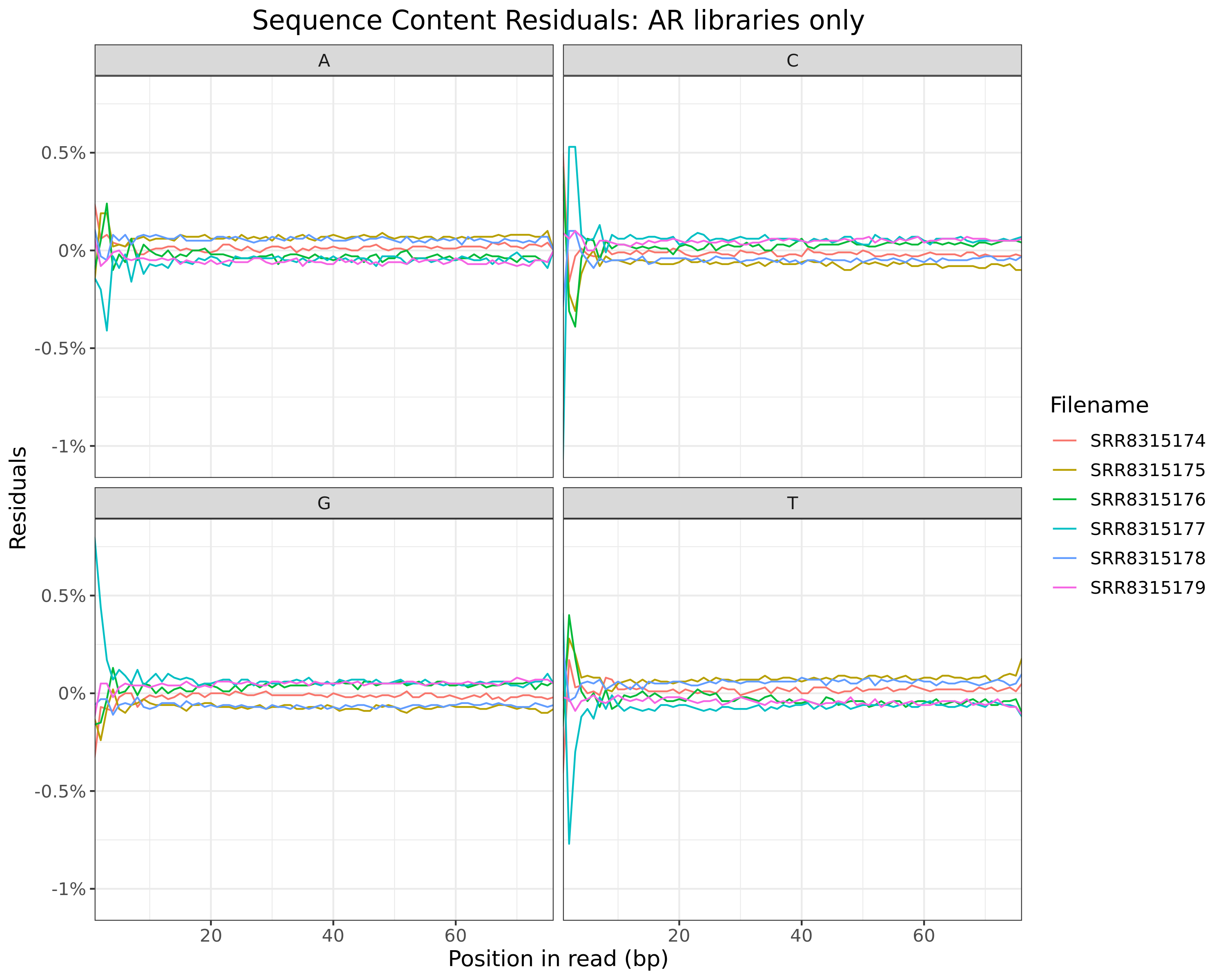
p <- plotSeqContent(fqc, plotType = "residuals", scaleColour = colours) +
ggtitle(glue("Sequence Content Residuals: {tgt} libraries only")) +
myTheme
png_out <- file.path(
d, glue("seq-content-residuals-{tgt}.png")
)
href <- str_extract(png_out, "assets.+")
png(filename = png_out, width = w, height = h, units = "in", res = 300)
print(p)
dev.off()
cp <- htmltools::em(
glue(
"
Residuals obtained when subtracting mean values at each position for
{tgt} libraries only.
"
)
)
htmltools::div(
htmltools::div(
id = glue("plot-seq-residuals-{tgt}"),
class = "section level4",
htmltools::h4(tgt),
htmltools::div(
class = "figure", style = "text-align: center",
htmltools::img(src = href, width = "100%"),
htmltools::tags$caption(cp)
)
)
)
}
)
)AR
ERa
H3K27ac
Input
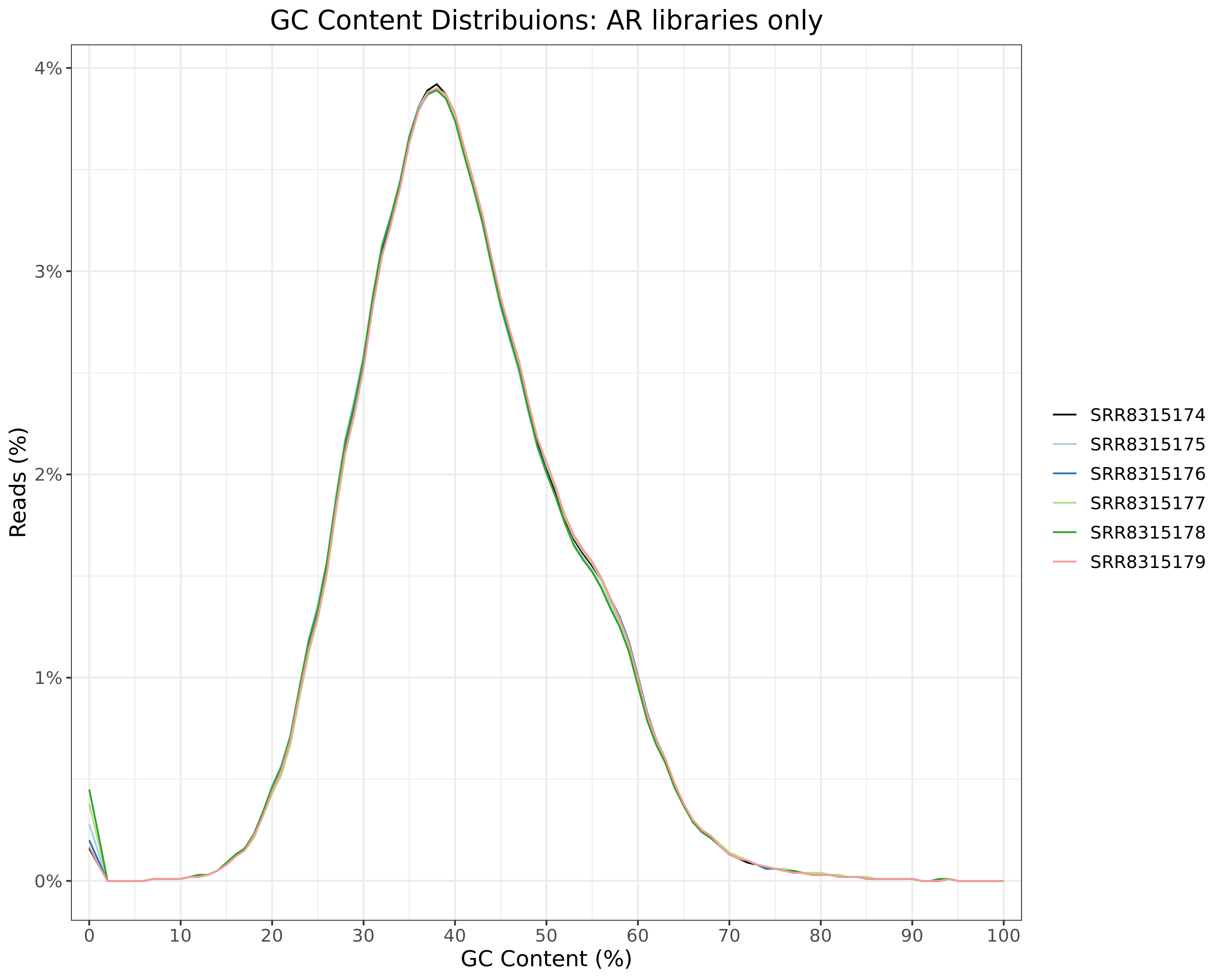
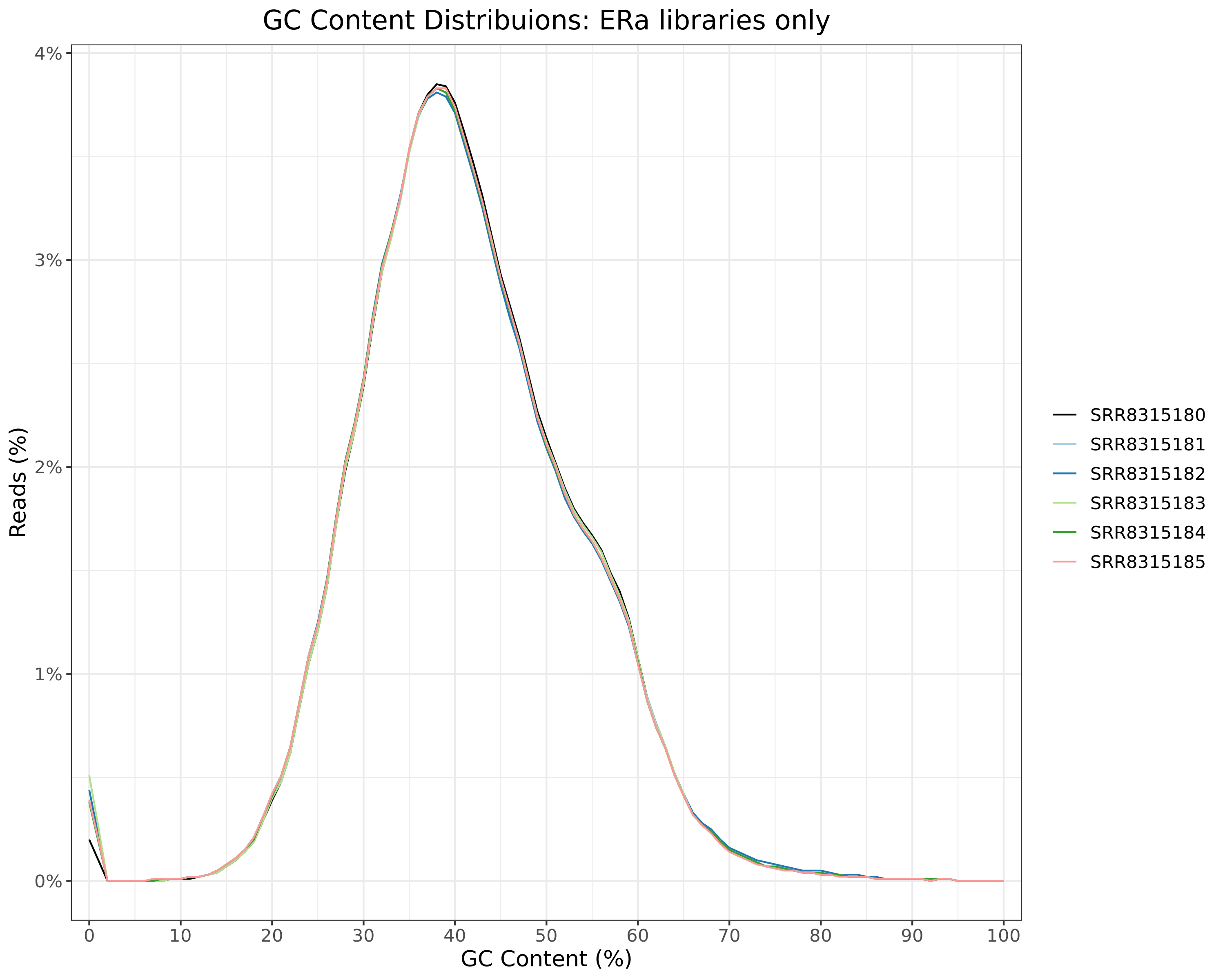
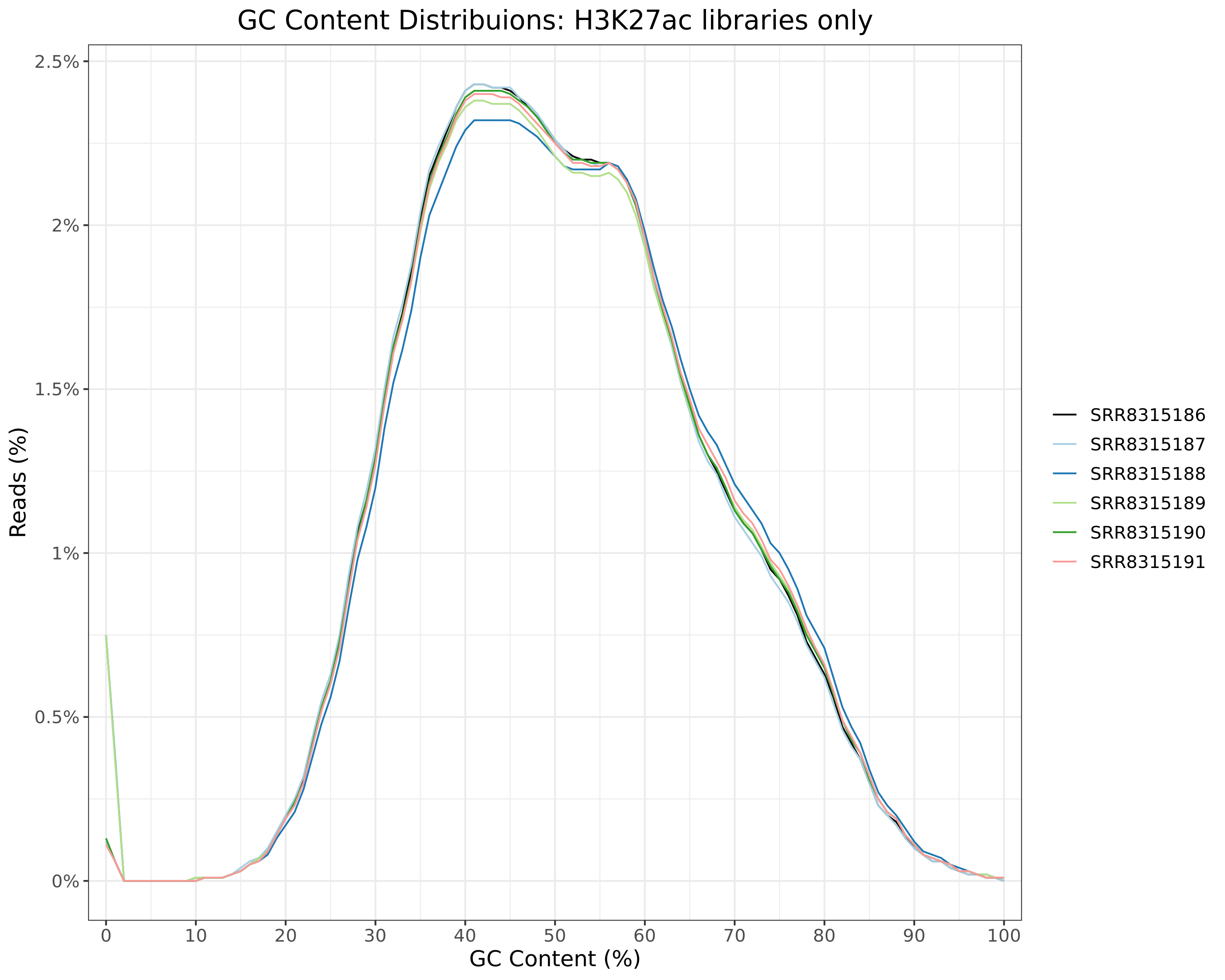
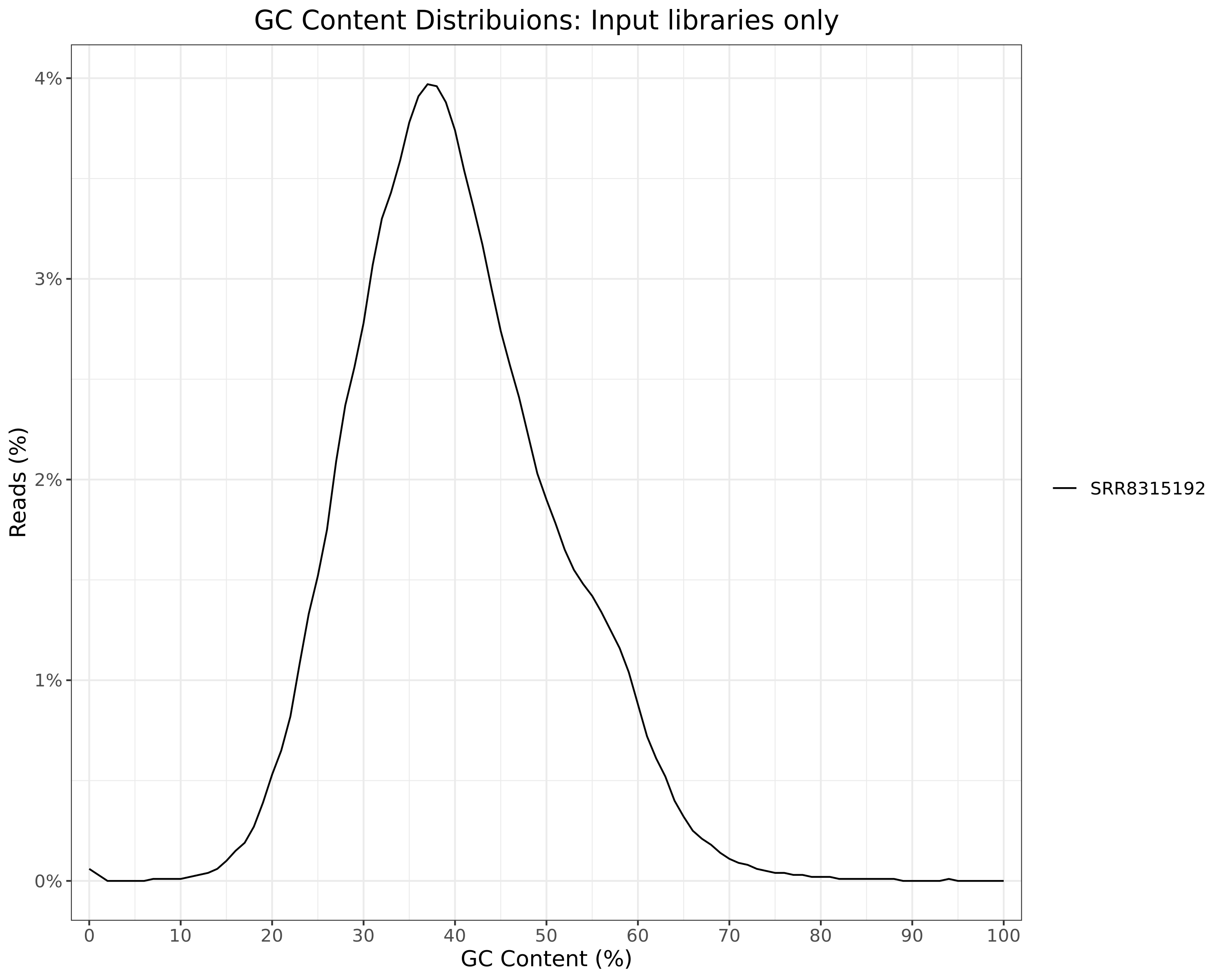
GC Content
All Libraries
plotGcContent(
  rawFqc, usePlotly = TRUE, plotType = "line", theoreticalGC = FALSE,
  scaleColour =  colours, plotlyLegend = TRUE, text = element_text(size = 13)
)
GC content distributions for all libraries
h <- knitr::opts_chunk$get("fig.height")
w <- knitr::opts_chunk$get("fig.width")
htmltools::tagList(
  samples %>%
    dplyr::filter(accession %in% names(rawFqc)) %>%
    split(.$target) %>%
    setNames(NULL) %>%
    lapply(
      function(x) {
        tgt <- unique(x$target)
        fqc <- rawFqc[x$accession]
        p <- plotGcContent(
          fqc, plotType = "line", theoreticalGC = FALSE, scaleColour = colours
        ) +
          ggtitle(glue("GC Content Distribuions: {tgt} libraries only")) +
          myTheme
        png_out <- file.path(
          d, glue("gc-content-{tgt}.png")
        )
        href <- str_extract(png_out, "assets.+")
        png(filename = png_out, width = w, height = h, units = "in", res = 300)
        print(p)
        dev.off()
        cp <- htmltools::em(
          glue("GC content distributions for {tgt} libraries only.")
        )
        htmltools::div(
          htmltools::div(
            id = glue("plot-gc_content-{tgt}"),
            class = "section level4",
            htmltools::h4(tgt),
            htmltools::div(
              class = "figure", style = "text-align: center",
              htmltools::img(src = href, width = "100%"),
              htmltools::tags$caption(cp)
            )
          )
        )
      }
    )
)
AR
ERa
H3K27ac
Input
Sequence Lengths
plotSeqLengthDistn(
  rawFqc, usePlotly = TRUE, plotType = "cdf", scaleColour = colours,
  plotlyLegend = TRUE, text = element_text(size = 13)
)
Cumulative Sequence Length distributions
Duplication Levels
plotDupLevels(
  rawFqc, usePlotly = TRUE, dendrogram = TRUE, heat_w = 20,
  text = element_text(size = 13)
)
Duplication levels as estimated by FastQC
Adapter Content
plotAdapterContent(
  rawFqc, usePlotly = TRUE, plotType = "line", scaleColour = colours,
  text = element_text(size = 13), plotlyLegend = TRUE
)
Total Adapter Content across all samples. If the total is below 0.1% an empty plot will be shown.
References
R version 4.2.3 (2023-03-15)
Platform: x86_64-conda-linux-gnu (64-bit)
locale: LC_CTYPE=en_AU.UTF-8, LC_NUMERIC=C, LC_TIME=en_AU.UTF-8, LC_COLLATE=en_AU.UTF-8, LC_MONETARY=en_AU.UTF-8, LC_MESSAGES=en_AU.UTF-8, LC_PAPER=en_AU.UTF-8, LC_NAME=C, LC_ADDRESS=C, LC_TELEPHONE=C, LC_MEASUREMENT=en_AU.UTF-8 and LC_IDENTIFICATION=C
attached base packages: stats, graphics, grDevices, utils, datasets, methods and base
other attached packages: Polychrome(v.1.5.1), htmltools(v.0.5.5), scales(v.1.2.1), ngsReports(v.2.0.0), patchwork(v.1.1.2), BiocGenerics(v.0.44.0), pander(v.0.6.5), reactable(v.0.4.4), here(v.1.0.1), yaml(v.2.3.7), glue(v.1.6.2), lubridate(v.1.9.2), forcats(v.1.0.0), stringr(v.1.5.0), dplyr(v.1.1.2), purrr(v.1.0.1), readr(v.2.1.4), tidyr(v.1.3.0), tibble(v.3.2.1), ggplot2(v.3.4.2) and tidyverse(v.2.0.0)
loaded via a namespace (and not attached): ggdendro(v.0.1.23), httr(v.1.4.6), sass(v.0.4.6), bit64(v.4.0.5), vroom(v.1.6.3), jsonlite(v.1.8.5), viridisLite(v.0.4.2), bslib(v.0.5.0), highr(v.0.10), stats4(v.4.2.3), GenomeInfoDbData(v.1.2.9), pillar(v.1.9.0), lattice(v.0.21-8), digest(v.0.6.31), RColorBrewer(v.1.1-3), XVector(v.0.38.0), colorspace(v.2.1-0), plyr(v.1.8.8), reactR(v.0.4.4), pkgconfig(v.2.0.3), zlibbioc(v.1.44.0), tzdb(v.0.4.0), timechange(v.0.2.0), farver(v.2.1.1), generics(v.0.1.3), IRanges(v.2.32.0), ellipsis(v.0.3.2), DT(v.0.28), cachem(v.1.0.8), withr(v.2.5.0), lazyeval(v.0.2.2), cli(v.3.6.1), magrittr(v.2.0.3), crayon(v.1.5.2), evaluate(v.0.21), fansi(v.1.0.4), MASS(v.7.3-60), tools(v.4.2.3), data.table(v.1.14.8), hms(v.1.1.3), lifecycle(v.1.0.3), plotly(v.4.10.2), S4Vectors(v.0.36.0), munsell(v.0.5.0), Biostrings(v.2.66.0), compiler(v.4.2.3), jquerylib(v.0.1.4), GenomeInfoDb(v.1.34.9), rlang(v.1.1.1), grid(v.4.2.3), RCurl(v.1.98-1.12), rstudioapi(v.0.14), htmlwidgets(v.1.6.2), crosstalk(v.1.2.0), labeling(v.0.4.2), bitops(v.1.0-7), rmarkdown(v.2.21), gtable(v.0.3.3), reshape2(v.1.4.4), R6(v.2.5.1), zoo(v.1.8-12), knitr(v.1.43), fastmap(v.1.1.1), bit(v.4.0.5), utf8(v.1.2.3), rprojroot(v.2.0.3), stringi(v.1.7.12), parallel(v.4.2.3), Rcpp(v.1.0.10), vctrs(v.0.6.3), scatterplot3d(v.0.3-44), tidyselect(v.1.2.0) and xfun(v.0.39)