ERa: MACS2 Summary
12 July, 2023
library(tidyverse)
library(magrittr)
library(rtracklayer)
library(glue)
library(pander)
library(scales)
library(plyranges)
library(yaml)
library(ngsReports)
library(ComplexUpset)
library(extraChIPs)
panderOptions("big.mark", ",")
panderOptions("missing", "")
panderOptions("table.split.table", Inf)
theme_set(
theme_bw() +
theme(
text = element_text(size = 13),
plot.title = element_text(hjust = 0.5)
)
)config <- read_yaml(here::here("config", "config.yml"))
macs2_path <- here::here(config$paths$macs2)
annotation_path <- here::here("output", "annotations")
macs2_cutoff <- config$params$macs2$callpeak %>%
str_extract("-[pq] [0-9\\.]+") %>%
str_remove_all("-") %>%
str_replace_all(" ", " < ")
if (is.na(macs2_cutoff)) macs2_cutoff <- "q < 0.05"target <- params$target
samples <- read_tsv(here::here(config$samples))
samples <- samples[samples$target == target,]
stopifnot(nrow(samples) > 0)
samples$treatment <- as.factor(samples$treatment)
treat_levels <- levels(samples$treatment)
treat_colours <- hcl.colors(max(3, length(treat_levels)), "Zissou 1")[seq_along(treat_levels)]
names(treat_colours) <- treat_levels
accessions <- samples$accessionsq <- file.path(annotation_path, "chrom.sizes") %>%
read_tsv(col_names = c("seqnames", "seqlengths")) %>%
mutate(isCircular = FALSE, genome = config$reference$name) %>%
as.data.frame() %>%
as("Seqinfo") %>%
sortSeqlevels()individual_peaks <- file.path(
macs2_path, accessions, glue("{accessions}_peaks.narrowPeak")
) %>%
importPeaks(seqinfo = sq) %>%
endoapply(sort) %>%
endoapply(names_to_column, var = "accession") %>%
endoapply(mutate, accession = str_remove(accession, "_peak_[0-9]+$")) %>%
endoapply(
mutate,
treatment = left_join(tibble(accession = accession), samples, by = "accession")$treatment
) %>%
setNames(accessions)
macs2_logs <- file.path(macs2_path, accessions, glue("{accessions}_callpeak.log")) %>%
importNgsLogs() %>%
dplyr::select(
-contains("file"), -outputs, -n_reads, -alt_fragment_length
) %>%
left_join(samples, by = c("name" = "accession")) %>%
mutate(
total_peaks = map_int(
name,
function(x) {
length(individual_peaks[[x]])
}
)
) QC Visualisations
This section provides a simple series of visualisations to aid in the detection of any problematic samples.
- Library Sizes: These are the total number of
alignments contained in each
bamfile, as passed tomacs2 callpeak(Zhang et al. 2008) - Peaks Detected: The number of peaks detected within each individual replicate are shown here, and provide clear guidance towards any samples where the IP may have been less successful, or there may be possible sample mis-labelling.
- Peak Widths: The peak widths for each sample are shown as a percentile to capture the overall distribution of widths
- FRIP: The Fraction of Reads in Peaks is a well-known ChIP-Seq metric for determining the success of the immuno-precipitation step (Landt et al. 2012)
- Cross Correlations: This provides an estimate of average fragment length and an additional guide as to the relative success of the IP step (Landt et al. 2012)
macs2_logs %>%
  mutate(target = target) %>%
  dplyr::select(
    sample = name, target, treatment,
    total_peaks,
    reads = n_tags_treatment, read_length = tag_length,
    fragment_length
  ) %>%
  setNames(
    names(.) %>% str_replace_all("_", " ") %>% str_to_title()
  ) %>%
  pander(
    justify = "lllrrrr",
    caption = glue(
      "*Summary of results for `macs2 callpeak` on individual {target} samples.",
      "Total peaks indicates the number retained after applying the cutoff ",
      "{macs2_cutoff} during the peak calling process.",
      "The fragment length as estimated by `macs2 predictd` is given in the final column.*",
      .sep = " "
    )
)| Sample | Target | Treatment | Total Peaks | Reads | Read Length | Fragment Length |
|---|---|---|---|---|---|---|
| SRR8315180 | ERa | E2 | 5,720 | 16,373,508 | 68 | 155 |
| SRR8315181 | ERa | E2 | 7,789 | 17,581,871 | 65 | 175 |
| SRR8315182 | ERa | E2 | 12,174 | 17,641,037 | 73 | 176 |
| SRR8315183 | ERa | E2DHT | 6,343 | 16,208,256 | 66 | 167 |
| SRR8315184 | ERa | E2DHT | 11,065 | 18,270,619 | 73 | 178 |
| SRR8315185 | ERa | E2DHT | 7,434 | 18,061,306 | 68 | 179 |
Library Sizes
macs2_logs %>%
  ggplot(
    aes(name, n_tags_treatment)
  ) +
  geom_col(position = "dodge", fill = "royalblue") +
  geom_hline(
    aes(yintercept = mn),
    data = . %>%
      group_by(treatment) %>%
      summarise(mn = mean(n_tags_treatment)),
    linetype = 2,
    col = "grey"
  ) +
  facet_grid(~treatment, scales = "free_x", space = "free_x") +
  scale_y_continuous(expand = expansion(c(0, 0.05)), labels = comma) +
  labs(
    x = "Sample", y = "Library Size"
  ) +
  ggtitle(
    glue("{target}: Library Sizes")
  )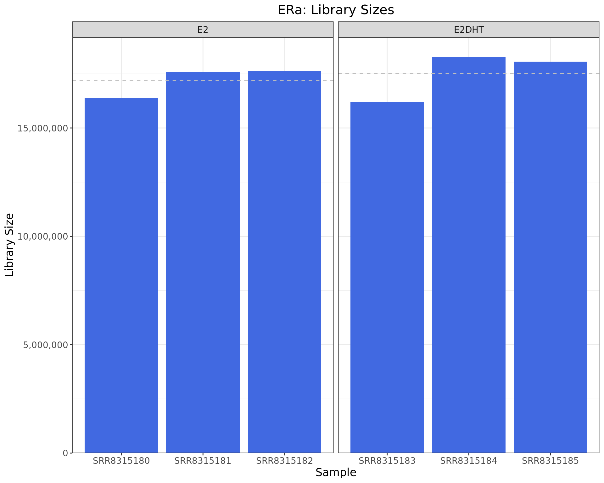
Library sizes for each ERa sample. The horizontal line indicates the mean library size for each treatment group.
Peaks Detected
macs2_logs %>%
  ggplot(
    aes(name, total_peaks)
  ) +
  geom_col(fill = "royalblue") +
  geom_label(
    aes(x = name, y = total_peaks, label = lab),
    data = . %>%
      dplyr::filter(total_peaks > 0) %>%
      mutate(
        lab = comma(total_peaks, accuracy = 1),
        total = total_peaks
      ),
    inherit.aes = FALSE, nudge_y = max(macs2_logs$total_peaks)/30,
    show.legend = FALSE
  ) +
  facet_grid(~treatment, scales = "free_x", space = "free_x") +
  scale_y_continuous(expand = expansion(c(0, 0.05)), labels = comma) +
  labs(
    x = "Sample",
    y = "Total Peaks",
    fill = "QC"
  ) +
  ggtitle(
    glue("{target}: Number of Peaks")
  )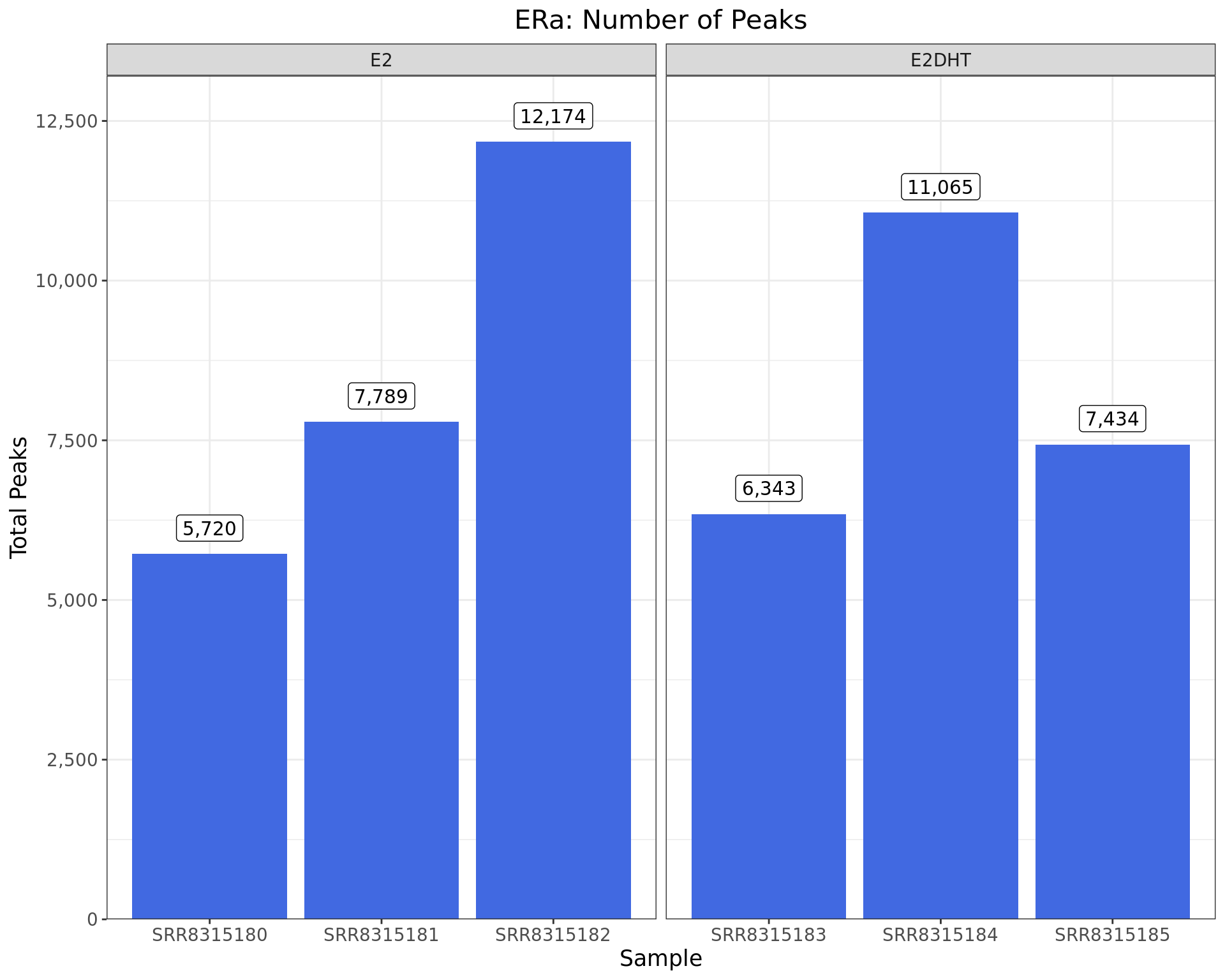
Peaks identified for each ERa sample. The number of peaks passing the inclusion criteria (q < 0.05) are shown as labels.
Peak Widths
individual_peaks %>%
  lapply(as_tibble, rangeAsChar = FALSE) %>%
  bind_rows() %>%
  arrange(accession, width) %>%
  summarise(
    n = dplyr::n(), .by = c(accession, treatment, width)
  ) %>%
  mutate(
    p = cumsum(n) / sum(n), .by = c(accession, treatment)
  ) %>%
  ggplot(aes(width, p, colour = accession, group = accession)) +
  geom_line() +
  coord_cartesian(
    xlim = quantile(width(unlist(individual_peaks)), c(0.005, 0.995))
  ) +
  scale_y_continuous(labels = percent, expand = expansion(c(0, 0.05)))  +
  labs(x = "Peak Width (bp)", y = "Percentile", colour = "Sample")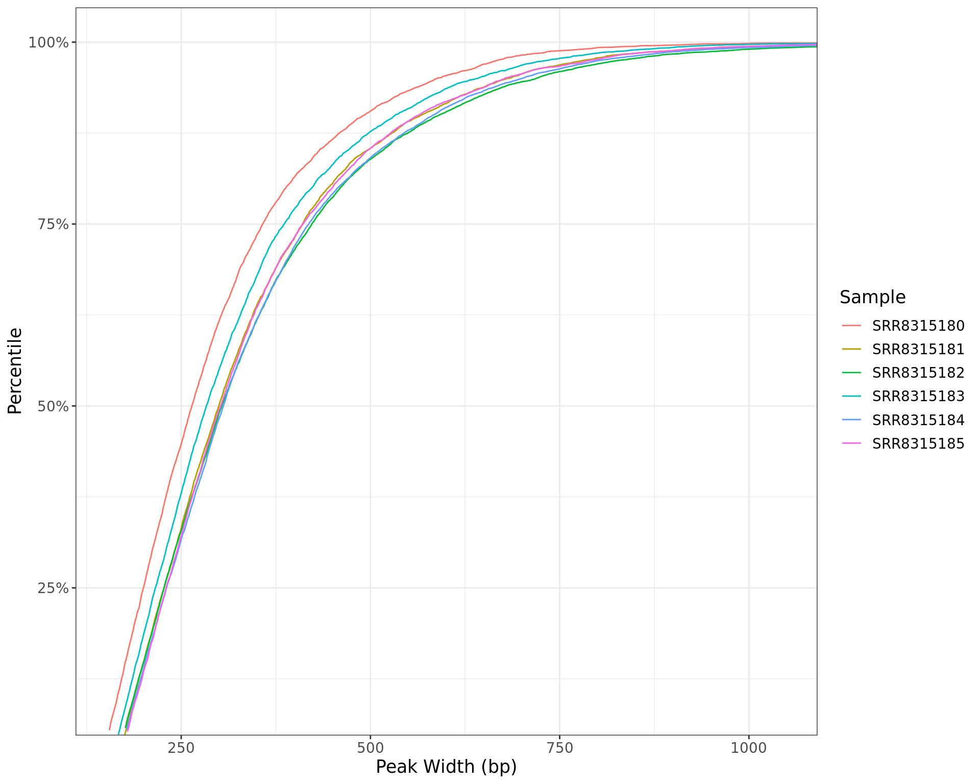
Peak widths for each sample shown as a cumulative percentile. The x-axis is restricted to the middle 99% of observed widths.
FRIP
here::here(macs2_path, accessions, paste0(accessions, "_frip.tsv")) %>%
  setNames(accessions) %>%
  lapply(read_tsv) %>%
  bind_rows(.id = "accession") %>%
  left_join(samples, by = "accession") %>%
  ggplot(aes(accession, frip)) +
  geom_col(fill = "royalblue") +
  geom_hline(yintercept = 0.01, colour = "grey", linetype = 2) +
  facet_wrap(~treatment, scales = "free_x") +
  labs(x = "Sample", y = "FRIP") +
  scale_y_continuous(expand = expansion(c(0, 0.05)), labels = percent) +
  ggtitle(
    glue("{target}: Fraction of Reads In Peaks")
  )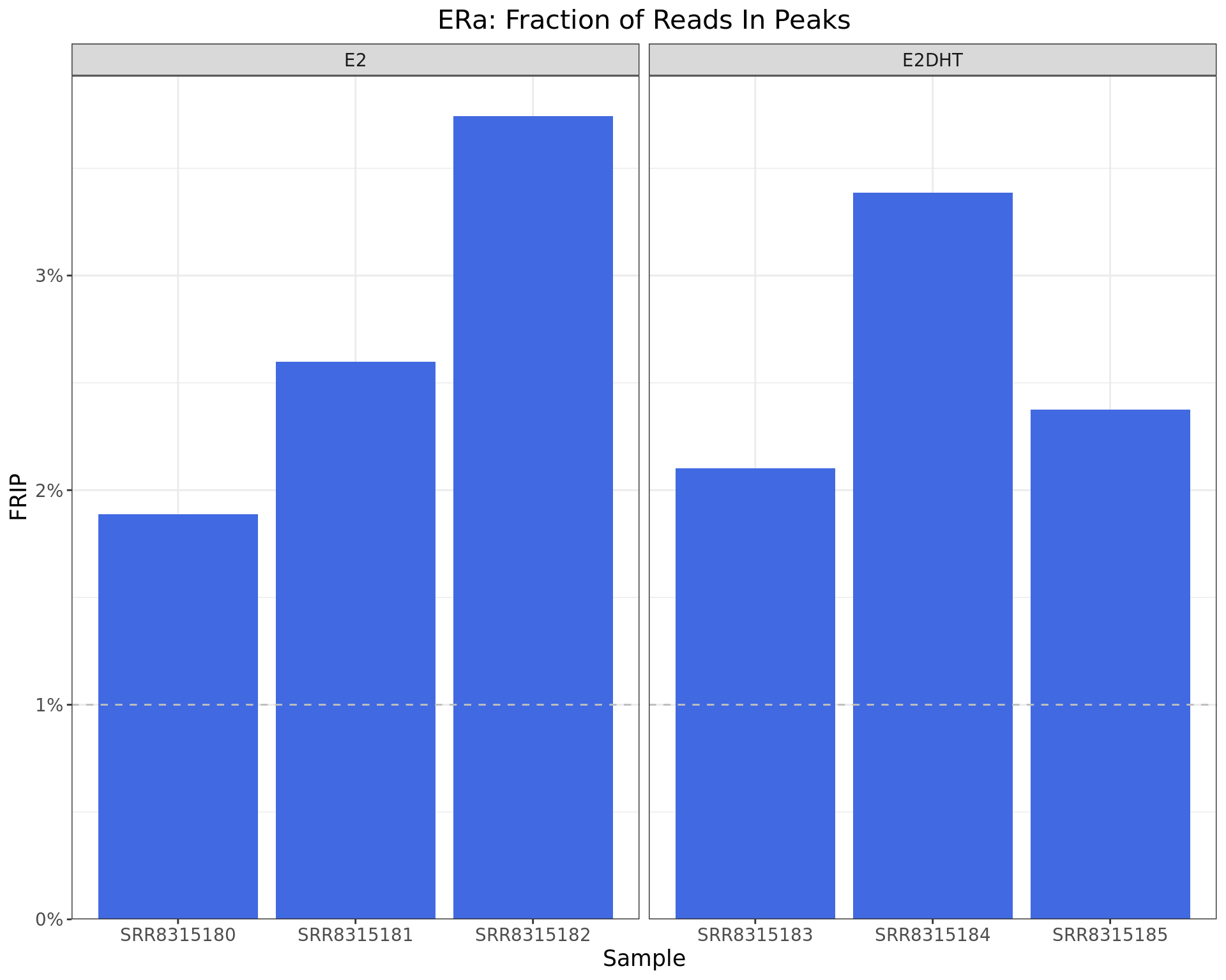
Fraction of Reads in Peaks. The common-use threshold of 1% is shown as the dashed line.
Cross Correlations
here::here(
  macs2_path, accessions, glue("{accessions}_cross_correlations.tsv")
  ) %>%
  lapply(read_tsv) %>%
  setNames(accessions) %>%
  bind_rows(.id = "accession") %>%
  left_join(samples, by = "accession") %>%
  ggplot(aes(fl, correlation, colour = treatment)) +
  geom_point(alpha = 0.1) +
  geom_smooth(se = FALSE, method = 'gam', formula = y ~ s(x, bs = "cs")) +
  geom_label(
    aes(label = fl),
    data = . %>%
      mutate(correlation = correlation + 0.025 * max(correlation)) %>%
      dplyr::filter(correlation == max(correlation), .by = accession),
    show.legend = FALSE, alpha = 0.7
  ) +
  facet_wrap(~accession) +
  scale_colour_manual(values = treat_colours) +
  labs(
    x = "Distance (bp)",
    y = "Cross Correlation",
    colour = "Treatment"
  ) +
  ggtitle(
    glue("{target}: Cross Correlations")
  )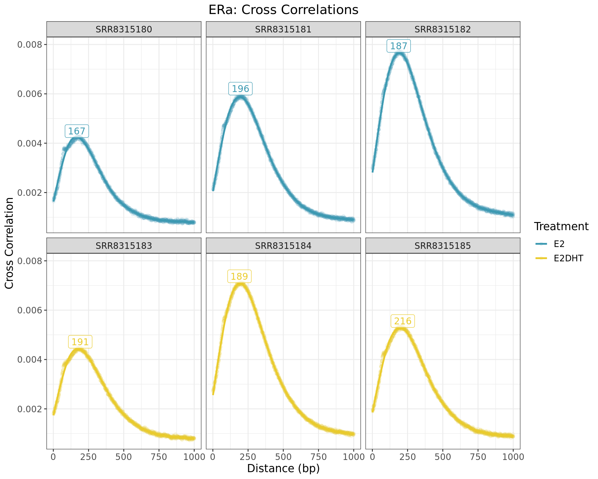
Cross correlations between reads. The distance corresponding to the maximum height provides a good estimate of the most common fragment length, with labels indicating these lengths. Relative heights between replicate samples also indicate the success of the immuno-precipitation. It is important to note that no black or grey lists were applied during data preparation, and a more rigorous analysis using the outputs generated here should do so.
Individual Replicates
A brief summary of all detected peaks for the given target within each replicate is shown using an UpSet plot below.
df <- individual_peaks %>%
  makeConsensus(var = "qValue") %>%
  as_tibble() %>%
  mutate(qValue = vapply(qValue, min, numeric(1)))
has_peaks <- vapply(accessions, function(x) sum(df[[x]]) > 0, logical(1)) %>%
  which() %>%
  names()
ql <- samples$accession %>%
  intersect(has_peaks) %>%
  lapply(
    function(x) {
      col <- as.character(dplyr::filter(samples, accession == x)$treatment)
      upset_query(
        set = x,
        fill = treat_colours[col]
      )
    }
  )
## Add the set of common peaks
if (nrow(dplyr::filter(df, if_all(all_of(accessions))))) {
  ql <- c(
    ql,
    list(
      upset_query(intersect = accessions, color = "royalblue", only_components = "intersections_matrix")
    )
  )
}
## Add the set of common peaks
if (nrow(dplyr::filter(df, if_all(all_of(accessions))))) {
  ql <- c(
    ql,
    list(
      upset_query(intersect = accessions, color = "royalblue", only_components = "intersections_matrix")
  )
  )
}
## Treatment specific common peaks
split_acc <- lapply(split(samples, samples$treatment), pull, accession)
if (length(split_acc) > 1) {
  treat_ql <- seq_along(split_acc) %>%
    lapply(
      function(i) {
        ids <- split_acc[[i]]
        others <- setdiff(unlist(split_acc), ids)
        nr <- df %>%
          dplyr::filter(!if_all(all_of(ids)), !if_any(all_of(others))) %>%
          nrow()
        if (nr > 10) return(ids)
        NULL
      }
    ) %>%
    .[vapply(., length, integer(1)) > 0] %>%
    lapply(
      function(x) {
        upset_query(intersect = x, color = "red", only_components = "intersections_matrix")
      }
    )
  if (length(treat_ql)) ql <- c(ql, treat_ql)
}
size <- get_size_mode('exclusive_intersection')
df %>%
  upset(
    intersect = accessions,
    base_annotations = list(
      `Peaks in Intersection` = intersection_size(
        text_mapping = aes(label = comma(!!size)),
        bar_number_threshold = 1, text_colors = "black",
        text = list(size = 3, angle = 90, vjust = 0.5, hjust = -0.1)
      ) +
        scale_y_continuous(expand = expansion(c(0, 0.2)), label = comma) +
        theme(
          panel.grid = element_blank(),
          axis.line = element_line(colour = "grey20"),
          panel.border = element_rect(colour = "grey20", fill =  NA)
        )
    ),
    annotations = list(
      qValue = ggplot(mapping = aes(y = qValue)) +
        geom_boxplot(na.rm = TRUE, outlier.colour = rgb(0, 0, 0, 0.2)) +
        coord_cartesian(ylim = c(0, quantile(df$qValue, 0.95))) +
        scale_y_continuous(expand = expansion(c(0, 0.05))) +
        ylab(expr(paste("Macs2 ", q[min]))) +
        theme(
          panel.grid = element_blank(),
          axis.line = element_line(colour = "grey20"),
          panel.border = element_rect(colour = "grey20", fill =  NA)
        )
    ),
    set_sizes = (
      upset_set_size() +
        geom_text(
          aes(label = comma(after_stat(count))),
          hjust = 1.1, stat = 'count', size = 3
        ) +
        scale_y_reverse(expand = expansion(c(0.2, 0)), label = comma) +
        ylab(glue("Macs2 Peaks")) +
        theme(
          panel.grid = element_blank(),
          axis.line = element_line(colour = "grey20"),
          panel.border = element_rect(colour = "grey20", fill =  NA)
        )
    ),
    queries = ql,
    min_size = 10,
    n_intersections = 35,
    keep_empty_groups = TRUE,
    sort_sets = FALSE
  ) +
  theme(
    panel.grid = element_blank(),
    panel.border = element_rect(colour = "grey20", fill =  NA),
    axis.line = element_line(colour = "grey20")
  ) +
  labs(x = "Intersection") +
  patchwork::plot_layout(heights = c(2, 3, 2))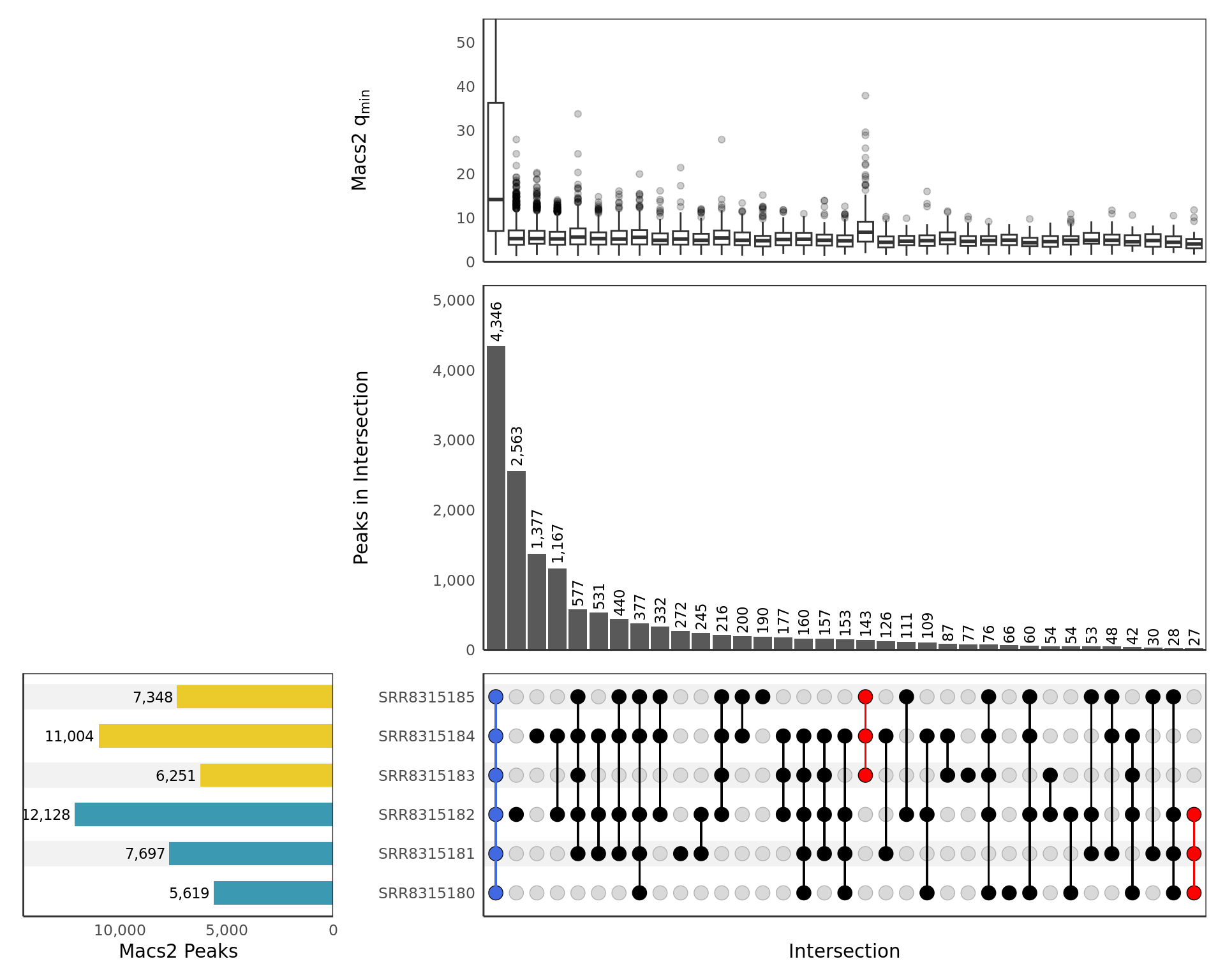
UpSet plot showing all samples. Any potential sample/treatment
mislabelling will show up clearly here as samples from each group may
show a preference to overlap other samples within the same treatment
group. Peaks shared between all samples, and exclusive to those within
each treatment group, are highlighted if found. Intersections are only
included if 10 or more sites are present. The top panel shows a boxplot
of the min \(q\)-values produced by
macs2 callpeak for each peak in the intersection as
representative of the sample with the weakest signal for each peak. The
y-axis for the top panel is truncated at the 95th percentile
of values.
Merged Replicates
In addition to the above sets of peaks, sets of peaks were called using merged samples within each treatment group.
merged_peaks <- file.path(
  macs2_path, target, glue("{treat_levels}_merged_peaks.narrowPeak")
) %>%
  importPeaks(seqinfo = sq) %>%
  setNames(treat_levels) %>%
  endoapply(plyranges::remove_names) %>%
  endoapply(sort)
merged_logs <- file.path(
  macs2_path, target, glue("{treat_levels}_merged_callpeak.log")
) %>%
  importNgsLogs() %>%
  dplyr::select(
    -contains("file"), -outputs, -n_reads, -alt_fragment_length
  ) %>%
  mutate(
    name = str_remove_all(name, "_merged"),
    total_peaks = map_int(
      name,
      function(x) {
        length(merged_peaks[[x]])
      }
    )
  )
merged_logs %>%
mutate(target = target) %>%
dplyr::select(
target, treatment = name,
total_peaks,
reads = n_tags_treatment, read_length = tag_length,
fragment_length
) %>%
setNames(
names(.) %>% str_replace_all("_", " ") %>% str_to_title()
) %>%
pander(
justify = "llrrrr",
caption = glue(
"*Summary of results for `macs2 callpeak` on merged {target} samples within treatment groups.",
"Total peaks indicates the number retained after applying the specified FDR",
"threshold during the peak calling process.",
"The fragment length as estimated by `macs2 predictd` is given in the final column.*",
.sep = " "
)
)| Target | Treatment | Total Peaks | Reads | Read Length | Fragment Length |
|---|---|---|---|---|---|
| ERa | E2 | 7,775 | 51,596,416 | 65 | 168 |
| ERa | E2DHT | 7,187 | 52,540,181 | 68 | 173 |
Merged Peak Overlaps
plotOverlaps(merged_peaks, set_col = treat_colours)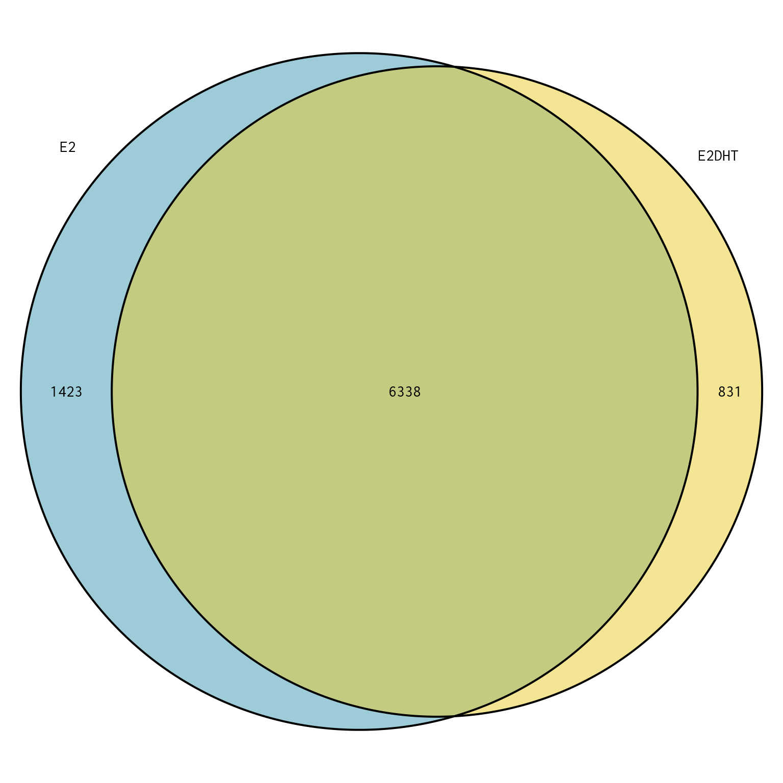
Overlap between peaks in each treatment-specific set of peaks called by merging replicates.
Merged Peak Widths
merged_peaks %>%
  lapply(as_tibble, rangeAsChar = FALSE) %>%
  bind_rows(.id = "treatment") %>%
  ggplot(aes(width, after_stat(density), fill = treatment, colour = treatment)) +
  geom_density(alpha = 0.3) +
  scale_x_log10(expand = expansion(c(0, 0.05))) +
  scale_y_continuous(expand = expansion(c(0, 0.05))) +
  scale_fill_manual(values = treat_colours) +
  scale_colour_manual(values = treat_colours) +
  labs(x = "Peak Width (bp)", y  = "Density", fill = "Treatment", colour = "Treatment") +
  ggtitle(
    glue("{target}: Peak Width Distributions for Merged Samples")
  )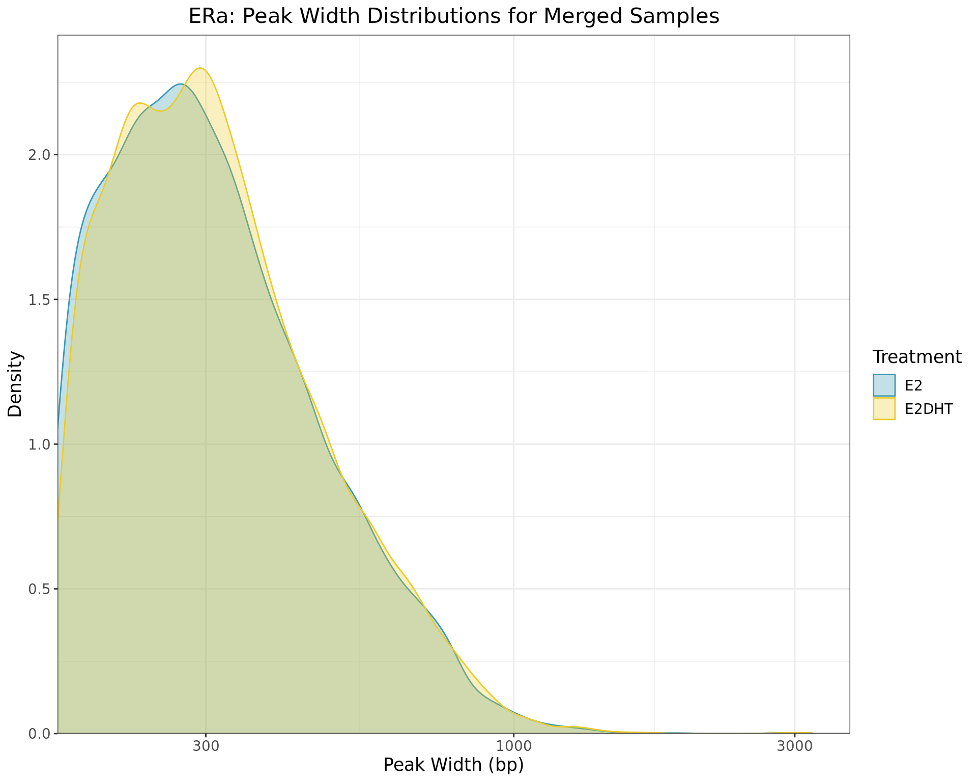
Distributions of peak widths when using merged samples for ERa within each treatment group
Merged Peaks By Individal Replicate
samples %>%
  split(.$treatment) %>%
  lapply(
    function(x) {
      trt <- unique(x$treatment)
      smp <- unique(x$accession)
      ol <- lapply(individual_peaks[smp], overlapsAny, subject = merged_peaks[[trt]])
      tbl <- lapply(ol, function(i) tibble(n = length(i), ol = sum(i), p = mean(i)))
      bind_rows(tbl, .id = "accession")
    }
  ) %>%
  bind_rows(.id = "treatment") %>%
  mutate(target = target) %>%
  ggplot() +
  geom_col(aes(accession, n), fill = "grey70", alpha = 0.7) +
  geom_col(aes(accession, ol), fill = "royalblue") +
  geom_label(
    aes(accession, 0.5 * ol, label = percent(p, 0.1)),
    fill = "white", alpha = 0.7
  ) +
  facet_wrap(~treatment, nrow = 1, scales = "free_x") +
  scale_y_continuous(expand = expansion(c(0, 0.05)), labels = comma) +
  labs(x = "Sample", y = "Individual Peaks")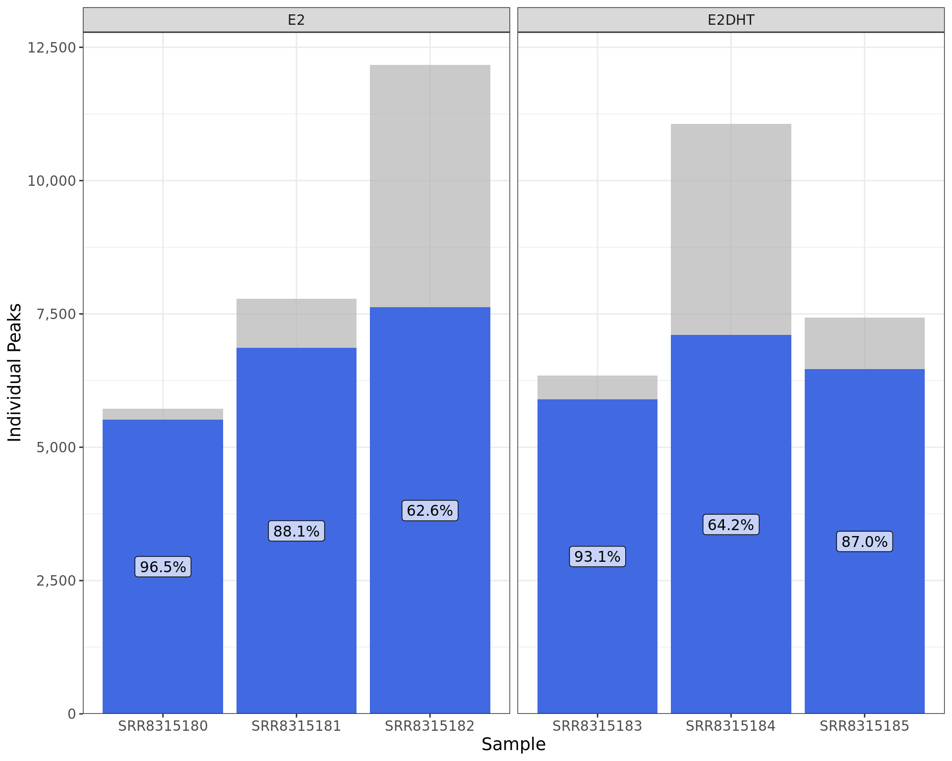
Peaks indentified using merged samples and the overlap with individual samples. Bar heights indicate the total number of peaks identified in each replicate, with the blue segments indicating those also identified when merging replicates.
Merged Peaks By Number Of Overlaps
samples %>%
  split(.$treatment) %>%
  lapply(
    function(x) {
      trt <- unique(x$treatment)
      acc <- unique(x$accession)
      ol <- lapply(acc, function(i) overlapsAny(merged_peaks[[trt]], individual_peaks[i]))
      names(ol) <- acc
      tbl <- as.matrix(as.data.frame(ol))
      counts <- table(rowSums(tbl))
      tibble(reps = names(counts), total = as.integer(counts))
    }
  ) %>%
  bind_rows(.id = "treatment") %>%
  mutate(reps = as.factor(reps)) %>%
  arrange(desc(reps)) %>%
  mutate(cumsum = cumsum(total), p = total / sum(total), .by = treatment) %>%
  mutate(y = cumsum - 0.5 * total) %>%
  ggplot(aes(treatment, total, fill = reps)) +
  geom_col() +
  geom_label(
    aes(treatment, y, label = percent(p, 0.1)),
    data = . %>% dplyr::filter(p > 0.05),
    fill = "white", alpha = 0.7
  ) +
  scale_y_continuous(expand = expansion(c(0, 0.05)), labels = comma) +
  scale_fill_viridis_d(direction = -1) +
  labs(x = "Treatment", y = "Merged Peaks", fill = "Overlapping\nReplicates")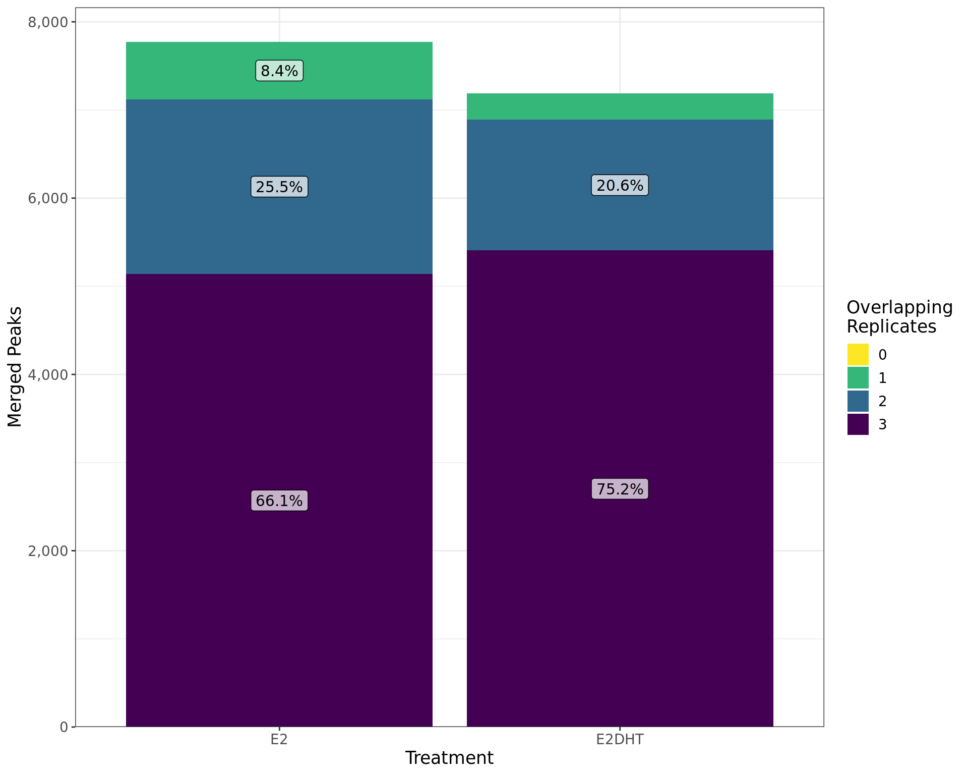
Treatment-specific peaks called by merging individual replcates are shown by the number of individual replicates they overlap. The percentages of peaks with each overlapping number are shown within each bar.
References
R version 4.2.3 (2023-03-15)
Platform: x86_64-conda-linux-gnu (64-bit)
locale: LC_CTYPE=en_AU.UTF-8, LC_NUMERIC=C, LC_TIME=en_AU.UTF-8, LC_COLLATE=en_AU.UTF-8, LC_MONETARY=en_AU.UTF-8, LC_MESSAGES=en_AU.UTF-8, LC_PAPER=en_AU.UTF-8, LC_NAME=C, LC_ADDRESS=C, LC_TELEPHONE=C, LC_MEASUREMENT=en_AU.UTF-8 and LC_IDENTIFICATION=C
attached base packages: stats4, stats, graphics, grDevices, utils, datasets, methods and base
other attached packages: extraChIPs(v.1.2.0), SummarizedExperiment(v.1.28.0), Biobase(v.2.58.0), MatrixGenerics(v.1.10.0), matrixStats(v.1.0.0), BiocParallel(v.1.32.5), ComplexUpset(v.1.3.3), ngsReports(v.2.0.0), patchwork(v.1.1.2), yaml(v.2.3.7), plyranges(v.1.18.0), scales(v.1.2.1), pander(v.0.6.5), glue(v.1.6.2), rtracklayer(v.1.58.0), GenomicRanges(v.1.50.0), GenomeInfoDb(v.1.34.9), IRanges(v.2.32.0), S4Vectors(v.0.36.0), BiocGenerics(v.0.44.0), magrittr(v.2.0.3), lubridate(v.1.9.2), forcats(v.1.0.0), stringr(v.1.5.0), dplyr(v.1.1.2), purrr(v.1.0.1), readr(v.2.1.4), tidyr(v.1.3.0), tibble(v.3.2.1), ggplot2(v.3.4.2) and tidyverse(v.2.0.0)
loaded via a namespace (and not attached): utf8(v.1.2.3), tidyselect(v.1.2.0), RSQLite(v.2.3.1), AnnotationDbi(v.1.60.0), htmlwidgets(v.1.6.2), grid(v.4.2.3), munsell(v.0.5.0), codetools(v.0.2-19), interp(v.1.1-4), DT(v.0.28), withr(v.2.5.0), colorspace(v.2.1-0), filelock(v.1.0.2), highr(v.0.10), knitr(v.1.43), rstudioapi(v.0.14), ggside(v.0.2.2), labeling(v.0.4.2), GenomeInfoDbData(v.1.2.9), polyclip(v.1.10-4), bit64(v.4.0.5), farver(v.2.1.1), rprojroot(v.2.0.3), vctrs(v.0.6.3), generics(v.0.1.3), lambda.r(v.1.2.4), xfun(v.0.39), biovizBase(v.1.46.0), timechange(v.0.2.0), csaw(v.1.32.0), BiocFileCache(v.2.6.0), R6(v.2.5.1), doParallel(v.1.0.17), clue(v.0.3-64), locfit(v.1.5-9.8), AnnotationFilter(v.1.22.0), bitops(v.1.0-7), cachem(v.1.0.8), DelayedArray(v.0.24.0), vroom(v.1.6.3), BiocIO(v.1.8.0), nnet(v.7.3-19), gtable(v.0.3.3), ensembldb(v.2.22.0), rlang(v.1.1.1), splines(v.4.2.3), GlobalOptions(v.0.1.2), lazyeval(v.0.2.2), dichromat(v.2.0-0.1), broom(v.1.0.5), checkmate(v.2.2.0), GenomicFeatures(v.1.50.2), backports(v.1.4.1), Hmisc(v.5.1-0), EnrichedHeatmap(v.1.27.2), tools(v.4.2.3), jquerylib(v.0.1.4), RColorBrewer(v.1.1-3), ggdendro(v.0.1.23), Rcpp(v.1.0.10), base64enc(v.0.1-3), progress(v.1.2.2), zlibbioc(v.1.44.0), RCurl(v.1.98-1.12), prettyunits(v.1.1.1), rpart(v.4.1.19), deldir(v.1.0-9), GetoptLong(v.1.0.5), zoo(v.1.8-12), ggrepel(v.0.9.3), cluster(v.2.1.4), here(v.1.0.1), data.table(v.1.14.8), futile.options(v.1.0.1), circlize(v.0.4.15), ProtGenerics(v.1.30.0), hms(v.1.1.3), evaluate(v.0.21), XML(v.3.99-0.14), VennDiagram(v.1.7.3), jpeg(v.0.1-10), gridExtra(v.2.3), shape(v.1.4.6), compiler(v.4.2.3), biomaRt(v.2.54.0), crayon(v.1.5.2), htmltools(v.0.5.5), mgcv(v.1.8-42), tzdb(v.0.4.0), Formula(v.1.2-5), DBI(v.1.1.3), tweenr(v.2.0.2), formatR(v.1.14), dbplyr(v.2.3.2), ComplexHeatmap(v.2.14.0), MASS(v.7.3-60), GenomicInteractions(v.1.32.0), rappdirs(v.0.3.3), Matrix(v.1.5-4.1), cli(v.3.6.1), parallel(v.4.2.3), Gviz(v.1.42.0), metapod(v.1.6.0), igraph(v.1.4.3), pkgconfig(v.2.0.3), GenomicAlignments(v.1.34.0), foreign(v.0.8-84), plotly(v.4.10.2), xml2(v.1.3.4), InteractionSet(v.1.26.0), foreach(v.1.5.2), bslib(v.0.5.0), XVector(v.0.38.0), VariantAnnotation(v.1.44.0), digest(v.0.6.31), Biostrings(v.2.66.0), rmarkdown(v.2.21), htmlTable(v.2.4.1), edgeR(v.3.40.0), restfulr(v.0.0.15), curl(v.5.0.1), Rsamtools(v.2.14.0), rjson(v.0.2.21), nlme(v.3.1-162), lifecycle(v.1.0.3), jsonlite(v.1.8.5), futile.logger(v.1.4.3), viridisLite(v.0.4.2), limma(v.3.54.0), BSgenome(v.1.66.3), fansi(v.1.0.4), pillar(v.1.9.0), lattice(v.0.21-8), KEGGREST(v.1.38.0), fastmap(v.1.1.1), httr(v.1.4.6), png(v.0.1-8), iterators(v.1.0.14), bit(v.4.0.5), ggforce(v.0.4.1), stringi(v.1.7.12), sass(v.0.4.6), blob(v.1.2.4), latticeExtra(v.0.6-30) and memoise(v.2.0.1)