Annotations
05 July, 2023
library(tidyverse)
library(magrittr)
library(rtracklayer)
library(glue)
library(pander)
library(scales)
library(yaml)
library(reactable)
library(htmltools)
library(plyranges)
library(GenomicInteractions)
library(extraChIPs)
library(GenomeInfoDb)
panderOptions("big.mark", ",")
panderOptions("missing", "")
panderOptions("table.split.table", Inf)
theme_set(
theme_bw() +
theme(plot.title = element_text(hjust = 0.5))
)
source(here::here("workflow", "scripts", "custom_functions.R"))
annotation_path <- here::here("output", "annotations")
all_out <- list(
chrom_sizes = file.path(annotation_path, "chrom.sizes"),
gene_regions = file.path(annotation_path, "gene_regions.rds"),
gtf_gene = file.path(annotation_path, "gtf_gene.rds"),
gtf_transcript = file.path(annotation_path, "gtf_transcript.rds"),
gtf_exon = file.path(annotation_path, "gtf_exon.rds"),
seqinfo = file.path(annotation_path, "seqinfo.rds"),
transcript_models = file.path(annotation_path, "trans_models.rds"),
tss = file.path(annotation_path, "tss.rds"),
colours = file.path(annotation_path, "colours.rds")
)config <- read_yaml(here::here("config", "config.yml"))
params <- read_yaml(here::here("config", "params.yml"))
colours <- read_yaml(here::here("config", "colours.yml"))
treat_levels <- config$comparisons$contrasts %>%
unlist() %>%
unique()
samples <- here::here(config$samples$file) %>%
read_tsv() %>%
mutate(
treat = factor(treat, levels = unique(c(treat_levels, treat))),
target = as.factor(target)
)
treat_levels <- levels(samples$treat)
has_external <- length(config$external$coverage) > 0
if (has_external) {
treat_levels <- c(
treat_levels,
lapply(config$external$coverage, names) %>% unlist()
) %>%
unique()
}Genome Annotations
Before analysing any datasets, annotations for the genome and transcriptome were checked and key objects were defined for consistent use throughout the workflow.
Genome Description
sq <- read_rds(file.path(annotation_path, "seqinfo.rds"))As the foundation for all annotation objects, the description of the
underlying genome is required as a Seqinfo object. For this
workflow, both the mitochondrial genome and any scaffolds are excluded,
giving only the autosomes and the X/Y chromosomes. This
Seqinfo object is added to all subsequent objects requiring
information about the underlying genome, such as a
GenomicRanges object.
Blacklisted Regions
blacklist <- import.bed(here::here(config$external$blacklist), seqinfo = sq)Blacklisted regions were supplied in the file
rconfig$external$blacklist.
Summary
blacklist %>%
  group_by(name) %>%
  summarise(
    n = n(),
    p = percent(sum(width) / sum(seqlengths(sq))),
    kb = sum(width) / 1e3,
    min = min(width) / 1e3,
    median = median(width) / 1e3,
    max = max(width) / 1e3
  ) %>%
  as_tibble() %>%
  dplyr::rename_all(str_to_title) %>%
  dplyr::rename(
    Type = Name,
    `Nbr Regions` = N,
    `% Genome` = P,
    `Total (kb)` = Kb,
    `Min (kb)` = Min,
    `Median (kb)` = Median,
    `Max (kb)` = Max
  ) %>%
  pander(
    caption = glue(
      "*Summary of genomic regions provided in the blacklist. ",
      "These regions will be excluded from all subsequent analyses.*"
    ),
    justify = "lrrrrrr"
)| Type | Nbr Regions | % Genome | Total (kb) | Min (kb) | Median (kb) | Max (kb) |
|---|---|---|---|---|---|---|
| High Signal Region | 583 | 8.7% | 269,778 | 1.1 | 13.4 | 30,590 |
| Low Mappability | 251 | 0.2% | 5,192 | 1.4 | 5.8 | 361.7 |
Breakdown
blacklist %>%
  as_tibble(rangeAsChar = FALSE) %>%
  group_by(seqnames) %>%
  summarise(blacklisted = sum(width)) %>%
  left_join(as_tibble(sq), by = "seqnames") %>%
  mutate(
    whitelisted = seqlengths - blacklisted,
    seqnames = factor(seqnames, levels = seqlevels(sq))
  ) %>%
  pivot_longer(
    ends_with("listed"), names_to = "category", values_to = "bp"
  ) %>%
  ggplot(aes(fct_rev(seqnames), bp/1e6, fill = fct_rev(category))) +
  geom_col() +
  coord_flip() +
  scale_y_continuous(expand = expansion(c(0, 0.05))) +
  scale_fill_manual(
    values = c(rgb(0.1, 0.3, 0.9), rgb(0.9, 0.2, 0.1))
  ) +
  labs(
    x = "Chromosome", y = "Length (Mb)", fill = "Status"
  )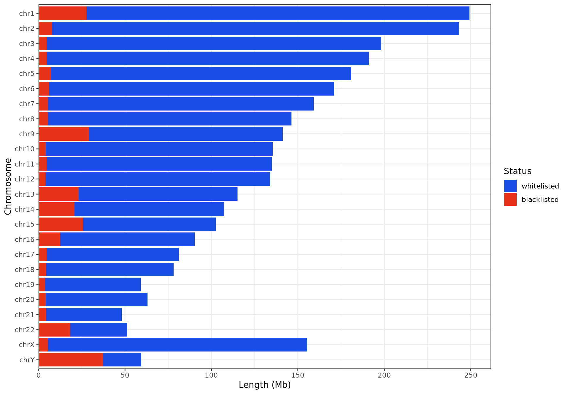
Breakdown of blacklisted regions by chromosome
Gene and Transcript Annotations
Basic Annotations
gtf_gene <- read_rds(file.path(annotation_path, "gtf_gene.rds"))
gtf_transcript <- read_rds(file.path(annotation_path, "gtf_transcript.rds"))
gtf_exon <- read_rds(file.path(annotation_path, "gtf_exon.rds"))- The complete set of genes, transcripts and exons was loaded from the
supplied
gtf, excluding mitochondrial features. - The previously generated
Seqinfowas also placed as the foundation of this annotation object, ensuring this propagates through all subsequent objects - Version numbers were removed from all gene, transcript and exon identifiers for convenience, with the minimal set of columns (type, gene_id, gene_type, gene_name, transcript_id, transcript_type, transcript_name and exon_id) retained.
- Visualisation using the Bioconductor package
Gvizrequires a specificGRangesstructure for gene and transcript models to be displayed. This object was created at this point so transcript models could be simply visualised throughout the workflow.
In total this annotation build contained 62,449 genes, 229,655 transcripts and 1,379,777 exons, after restricting the dataset to the autosomes and sex chromosomes.
Gene-Centric Regions
gene_regions <- read_rds(file.path(annotation_path, "gene_regions.rds"))
regions <- vapply(gene_regions, function(x) unique(x$region), character(1))
missing_reg_col <- setdiff(names(regions), names(colours$regions))
if (length(missing_reg_col) > 0) {
  def_reg_cols <- c(
    promoter = "#FF3300", upstream_promoter = "#E1EE05", exon = "#7EDD57",
    intron = "#006600", proximal_intergenic = "#000066", distal_intergenic = "#551A8B"
  )
  colours$regions[missing_reg_col] <- def_reg_cols[missing_reg_col]
}
region_cols <- unlist(colours$regions) %>%
  setNames(regions[names(.)])
Using the provided GTF, unique gene and
transcript-centric features were also defined using
defineRegions(), and will be treated as annotated regions
throughout the workflow. The regions are:
- Promoters (-1500/+500bp)
- Upstream Promoters (> 1500bp; < 5000bp)
- Exons
- Introns
- Intergenic regions within 10kb of a gene
- Intergenic regions >10kb from any defined genes
Colours were also defined for each of these regions for consistent visualisation.
In addition, TSS regions were defined as a separate object given each TSS has single-base width. With the exception of TSS and Promoters, these features were non-overlapping and defined in a hierarchical, un-stranded manner. TSS regions represent the individual start sites for each transcript, and given that many transcripts can originate from the same TSS, this is somewhat smaller than the number of actual transcripts defined in the GTF.
cp <- em(
  glue(
    "
  Summary of gene-centric regions defined as a key annotation set.
  Colours used throughout the workflow for each region are indicated in the
  first column, with other summary statistics making up the rest of the table.
  "
  )
)
tbl <- gene_regions %>%
  lapply(
    function(x){
      tibble(
        n = length(x),
        width = sum(width(x)),
        region = unique(x$region)
      )
    }
  ) %>%
  bind_rows() %>%
  mutate(
    width = width / 1e6,
    mn = 1e3*width/n,
    region = fct_inorder(region),
    `% Genome` = width / sum(width),
  ) %>%
  rename_all(str_to_title) %>%
  mutate(Guide = region_cols[Region]) %>%
  dplyr::select(
    Guide, Region, N, Width, Mn, `% Genome`
  ) %>%
  reactable(
    searchable = FALSE, filterable = FALSE,
    columns = list(
      Guide = colDef(
        maxWidth = 50,
        style = function(value) list(background = value),
        cell = function(value) "",
        name = ""
      ),
      Region = colDef(minWidth = 200),
      N = colDef(
        maxWidth = 150,
        cell = function(value) comma(value, 1)
      ),
      Width = colDef(
        name = "Total Width (Mb)",
        cell = function(value) sprintf("%.1f", value)
      ),
      Mn = colDef(
        name = "Average Width (kb)",
        cell = function(value) sprintf("%.2f", value)
      ),
      "% Genome" = colDef(
        cell = function(value) percent(value, 0.1)
      )
    )
  )
div(class = "table",
  div(class = "table-header",
      div(class = "caption", cp),
      tbl
  )
)
Summary
gene_regions %>%
  lapply(select, region) %>%
  GRangesList() %>%
  unlist() %>%
  mutate(region = factor(region, levels = regions)) %>%
  setNames(NULL) %>%
  plotPie(
    fill = "region", scale_by = "width", scale_factor = 1e6,
    total_glue = "{comma(N, 0.1)}Mb", total_size = 4.5,
    cat_glue = "{str_wrap(.data[[fill]], 10)}\n{comma(n, 0.1)}Mb\n({percent(p, 0.1)})",
    cat_alpha = 0.8, cat_adj = 0.1, cat_size = 3.5
  ) +
  scale_fill_manual(values = region_cols) +
  theme(legend.position = "none")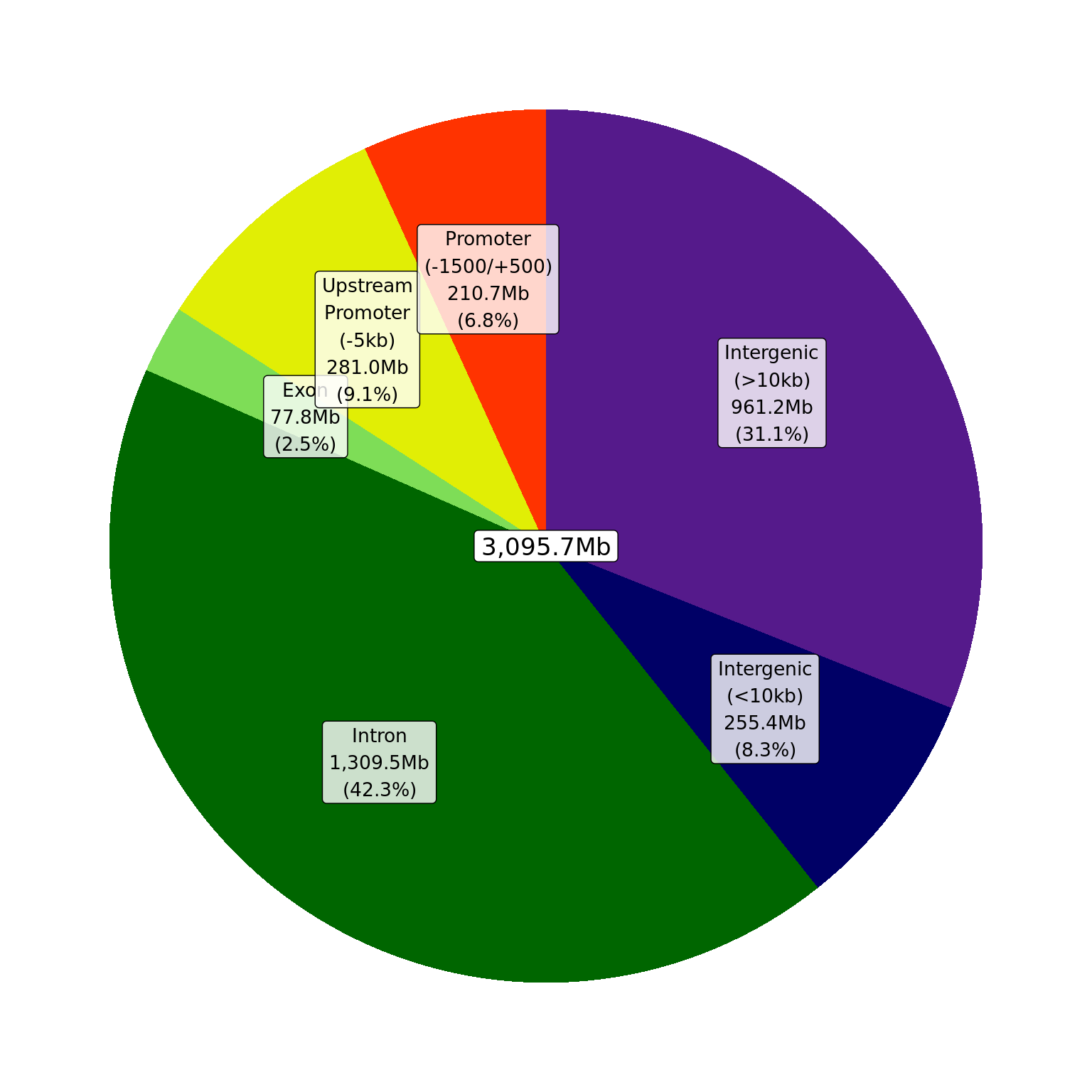
Summary of gene-centric regions using defineRegions()
and the supplied GTF. Percentages represent the amount of the genome
allocated to each region with total widths shown in Mb. Blacklisted
regions were not considered for this step of the annotation.
Example
id <- sort(gtf_gene$gene_id)[[1]]gr <- subset(gtf_gene, gene_id == id) %>%
resize(width = width(.) + 2.4e4, fix = 'center') %>%
unstrand()
ft <- gene_regions %>%
lapply(subsetByOverlaps, gr) %>%
lapply(select, region) %>%
lapply(intersectMC, gr) %>%
GRangesList() %>%
unlist() %>%
setNames(c()) %>%
subset(region != "TSS") %>%
sort()
df <- list(
gtf_transcript %>%
subsetByOverlaps(gr) %>%
as_tibble(rangeAsChar = FALSE),
gtf_exon %>%
subsetByOverlaps(gr) %>%
as_tibble(rangeAsChar = FALSE)
) %>%
bind_rows() %>%
mutate(
transcript_name = as.factor(transcript_name)
)
df %>%
ggplot(aes(x = start, y = as.integer(transcript_name))) +
geom_rect(
aes(
xmin = start, xmax = end,
ymin = 0, ymax = Inf,
fill = region
),
data = ft %>%
as.data.frame() %>%
mutate(region = fct_inorder(region) ),
inherit.aes = FALSE,
alpha = 0.6
) +
geom_segment(
aes(
x = start, xend = end,
y = as.integer(transcript_name),
yend = as.integer(transcript_name)
),
data = . %>%
dplyr::filter(type == "transcript")
) +
geom_segment(
aes(
x = mid, xend = mid_offset,
y = as.integer(transcript_name),
yend = as.integer(transcript_name)
),
data = gtf_transcript %>%
subsetByOverlaps(gr) %>%
select(transcript_name) %>%
setdiffMC(gtf_exon) %>%
as.data.frame() %>%
mutate(transcript_name = vctrs::vec_proxy(transcript_name)) %>%
unnest(transcript_name) %>%
dplyr::filter(width > 600) %>%
mutate(
mid = end - 0.5*width,
mid_offset = ifelse(strand == "+", mid + 50, mid - 50),
transcript_name = factor(transcript_name, levels = levels(df$transcript_name))
),
arrow = arrow(angle = 40, length = unit(0.015, "npc"))
) +
geom_rect(
aes(
xmin = start, xmax = end,
ymin = as.integer(transcript_name) - 0.2,
ymax = as.integer(transcript_name) + 0.2
),
data = . %>%
dplyr::filter(type == "exon"),
fill = "blue", colour = "blue"
) +
coord_cartesian(xlim = c(start(gr), end(gr))) +
scale_x_continuous(
labels = comma, expand = expansion(c(0, 0))
) +
scale_y_continuous(
breaks = seq_along(levels(df$transcript_name)),
labels = levels(df$transcript_name),
expand = expansion(c(-0.05, 0.05))
) +
scale_fill_manual(values = region_cols) +
labs(
x = as.character(seqnames(gr)), y = "Transcript", fill = "Feature"
) +
theme(
panel.grid = element_blank()
)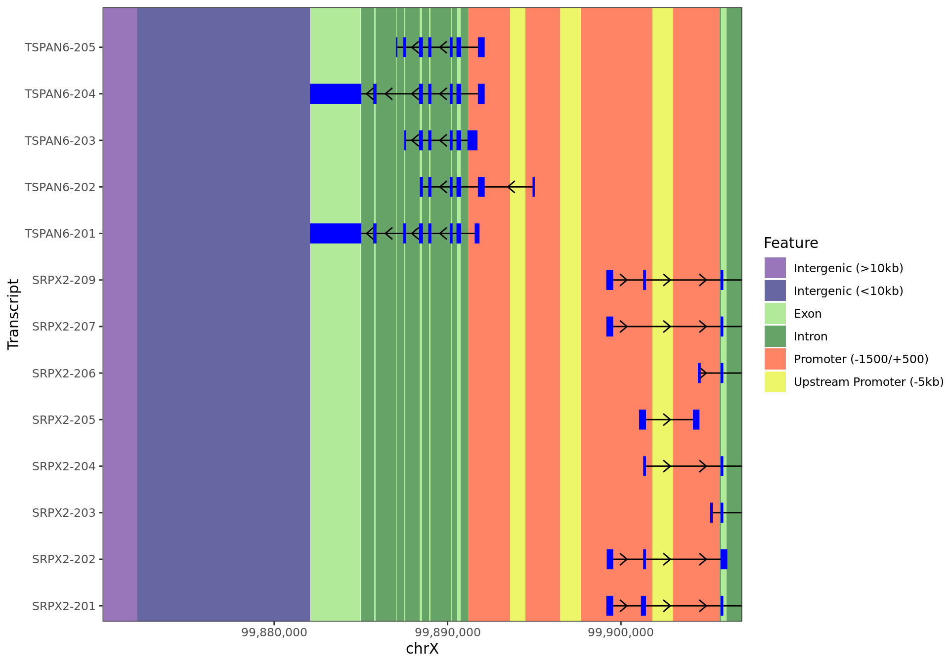
12kb region surrounding TSPAN6 showing all annotated regions.
External Features
feat_path <- here::here(config$external$features)
external_features <- list(features = c())
has_features <- FALSE
if (length(feat_path) > 0) {
  stopifnot(file.exists(feat_path))
  external_features <- suppressWarnings(
    import.gff(feat_path, genome = sq)
  )
  mcols(external_features) <- cbind(
    mcols(external_features),
    gene_regions %>%
      lapply(function(x) propOverlap(external_features, x)) %>%
      as("DataFrame")
  )
  keep_cols <- !vapply(
    mcols(external_features), function(x) all(is.na(x)), logical(1)
  )
  mcols(external_features) <- mcols(external_features)[keep_cols]
  has_features <- TRUE
}
feat_col <- colours$features
feat_levels <- unique(external_features$feature)
missing_feat_col <- setdiff(feat_levels, names(feat_col))
if (length(missing_feat_col) > 0) {
if (!"no_feature" %in% feat_levels)
missing_feat_col <- c(missing_feat_col, "no_feature")
n <- length(missing_feat_col)
feat_col[missing_feat_col] <- hcl.colors(max(9, n), "Spectral")[seq_len(n)]
}
colours$features <- feat_colExternal features were compared to the gene-centric annotations.
external_features %>%
  as_tibble() %>%
  dplyr::select(range, feature, all_of(names(gene_regions))) %>%
  pivot_longer(
    cols = all_of(names(gene_regions)), names_to = "region", values_to = "p"
  ) %>%
  mutate(region = regions[region]) %>%
  plotSplitDonut(
    inner = "feature", outer = "region", scale_by = "p", scale_factor = 1,
    inner_palette = colours$feature, outer_palette = region_cols,
    inner_glue = "{str_wrap(.data[[inner]], 10)}\n{comma(n, 1)}\n{percent(p,0.1)}",
    outer_glue = "{str_wrap(.data[[outer]], 15)}\n{percent(p,0.1)}",
  )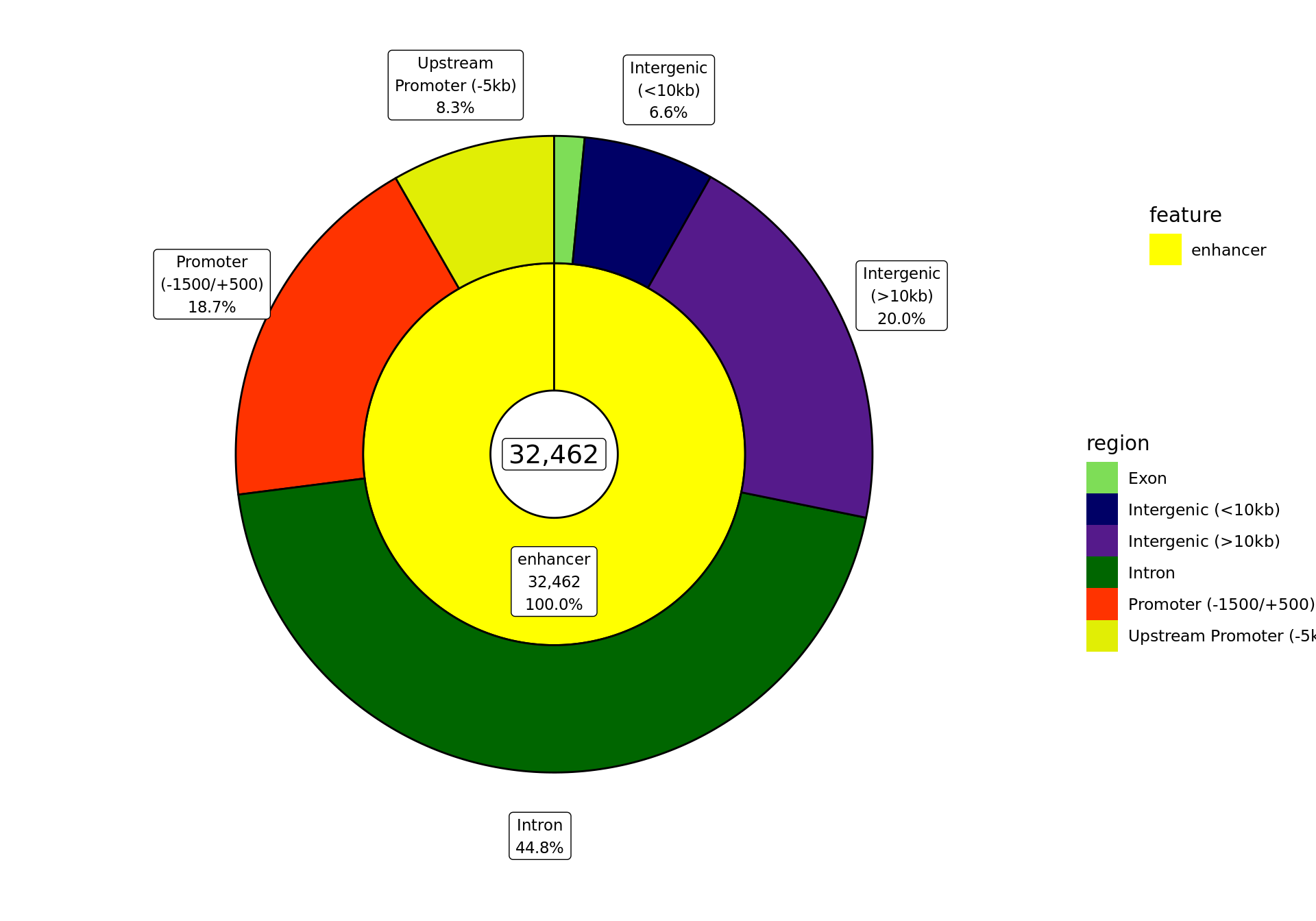
The proportion of the ranges provided as external features in the file enhancer_atlas_2.0_zr75.gtf.gz, and which overlap the gene-centric regions defined above. Values were estimated using the proportion of bases within each feature that overlap each of the regions.
cp <- em(
  glue(
      "Summary of external features provided in the file ",
      "{basename(config$external$feature)}. All peaks and windows will be ",
      "compared to these throughout the workflow. The colours defined for each ",
      "feature is show as a guide on the left."
    )
)
tbl <- external_features %>%
  group_by(feature) %>%
  summarise(
    N = n(),
    Width = sum(width/1e3),
    med = median(width/1e3),
    range = glue("[{round(min(width/1e3), 1)}, {round(max(width/1e3), 1)}]")
  ) %>%
  as_tibble() %>%
  mutate(
    guide = unlist(feat_col)[feature],
    feature = factor(feature, levels = names(feat_col)) %>%
      fct_relabel(str_sep_to_title)
  ) %>%
  arrange(feature) %>%
  dplyr::select(guide, everything()) %>%
  reactable(
    filterable = FALSE, searchable = FALSE,
    columns = list(
      guide = colDef(
        maxWidth = 40,
        style = function(value) list(background = value),
        cell = function(value) "",
        name = ""
      ),
      feature = colDef(
        name = "Feature",
        footer = htmltools::tags$b("Total")
      ),
      N = colDef(
        cell = function(value) comma(value, 1),
        footer = htmltools::tags$b(comma(sum(.$N)))
      ),
      Width = colDef(
        name = "Total Width (kb)",
        cell = function(value) comma(value, 1),
        footer = htmltools::tags$b(comma(sum(.$Width), 1))
      ),
      med = colDef(
        name = "Median Width (kb)",
        cell = function(value) sprintf("%.2f", value)
      ),
      range = colDef(name = "Size Range (kb)", align = "right")
    )
  )
div(class = "table",
  div(class = "table-header",
      div(class = "caption", cp),
      tbl
  )
)HiC Data
No HiC Data was supplied as an input.
Colour Schemes
## qc_colours need to have `Pass` and `Fail`
missing_qc_cols <- setdiff(c("pass", "fail"), names(colours$qc))
if ("pass" %in% missing_qc_cols) colours$qc$pass <- "#0571B0" # Blue
if ("fail" %in% missing_qc_cols) colours$qc$fail <- "#CA0020" # Red
colours$qc <- colours$qc[c("pass", "fail")]

## The colours specified as treat_colours should contain all treat_levels + Input
## If Input is missing, set to #33333380 ('grey20' + alpha = 50)
## This should be a standard chunk for all workflows
missing_treat_cols <- setdiff(
  c("Input", treat_levels), names(colours$treat)
)
if (length(missing_treat_cols) > 0) {
  if ("Input" %in% missing_treat_cols)
    colours$treat$Input <- "#33333380"
  ## Automatically sample from the viridis palette if no colour is assigned
  colours$treat[setdiff(missing_treat_cols, "Input")] <- hcl.colors(
    length(setdiff(missing_treat_cols, "Input"))
  )
}

## Direction colours always need up, down, unchanged & undetected
missing_dir_cols <- setdiff(
  c("up", "down", "unchanged", "undetected", "ambiguous"),
  names(colours$direction)
)
if (length(missing_dir_cols) > 0) {
  def_dir_cols <- c(
    up = "#CA0020", down = "#0571B0",
    unchanged = "#7F7F7F", undetected = "#E5E5E5",
    ambiguous = "#000000"
  )
  colours$direction[missing_dir_cols] <- def_dir_cols[missing_dir_cols]
}

## Heatmap gradients
if (length(colours$heatmaps) < 2) {
  colours$heatmaps <- unique(c(colours$heatmaps,  c("white", "red")))
}


write_rds(colours, all_out$colours, compress = "gz")
Colours were checked where provided and any missing colours were
automatically assigned. These colour schemes are shown below and will be
propagated through all steps of the workflow. To change any colours,
simply add them to config/rmarkdown.yml.
QC
.plotScheme(colours$qc , xlab = "QC Category") 
Treatment Groups
.plotScheme(colours$treat, xlab = "Treatment")
Regions
.plotScheme(colours$regions, xlab = "Regions")
Features
.plotScheme(feat_col, xlab = "Feature")
Direction
.plotScheme(colours$direction, xlab = "Direction")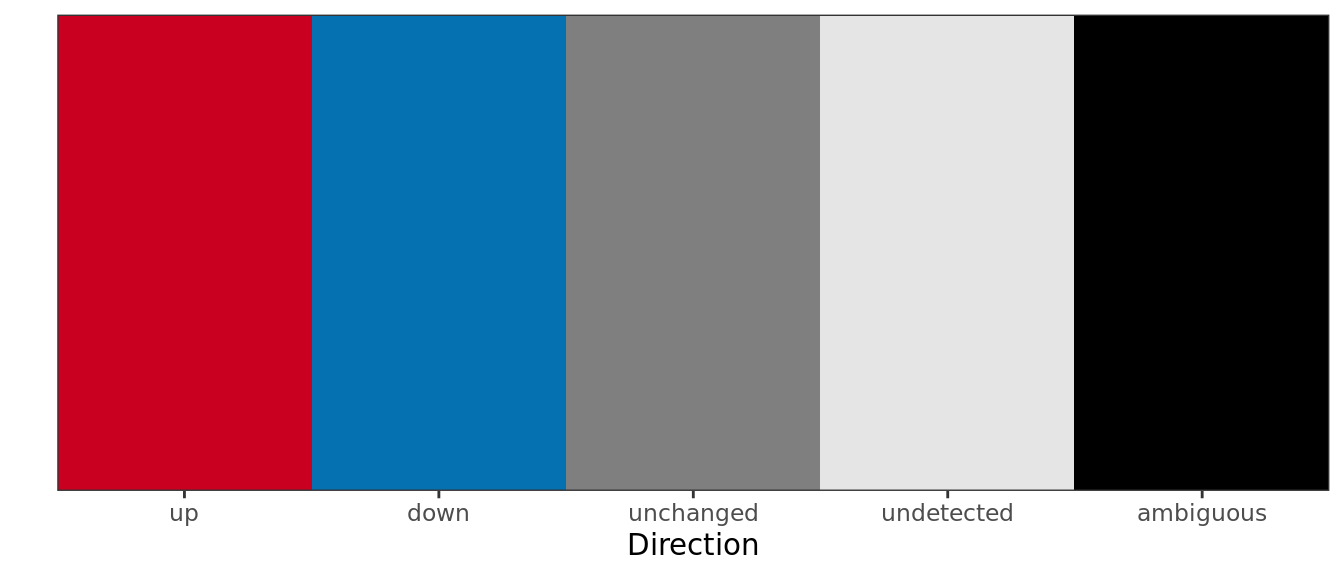
Heatmap Gradient
colorRampPalette(colours$heatmaps)(11) %>%
  setNames(percent(seq(0, 1, length.out = 11))) %>%
  as.list() %>%
  .plotScheme(xlab = "% Of Signal")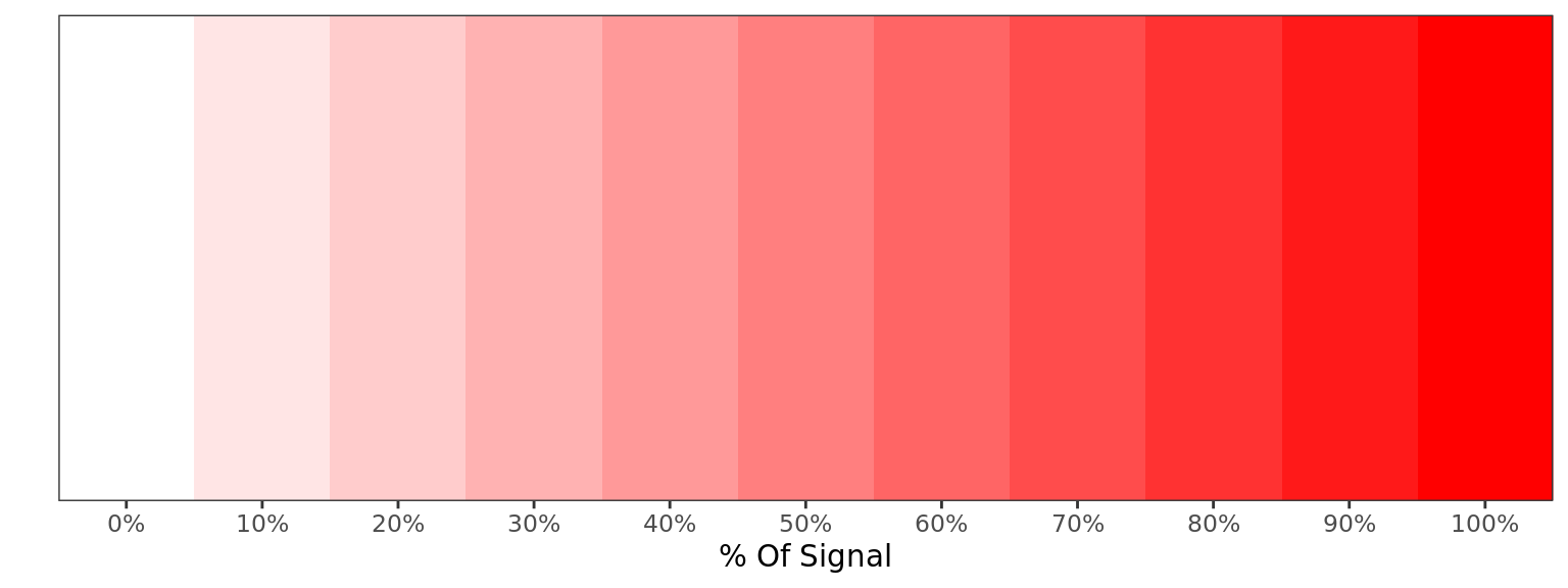
Data Export
During setup of all required annotations, the following files were exported:
- chrom_sizes: GRAVI_PRJNA509779/output/annotations/chrom.sizes
- gene_regions: GRAVI_PRJNA509779/output/annotations/gene_regions.rds
- gtf_gene: GRAVI_PRJNA509779/output/annotations/gtf_gene.rds
- gtf_transcript: GRAVI_PRJNA509779/output/annotations/gtf_transcript.rds
- gtf_exon: GRAVI_PRJNA509779/output/annotations/gtf_exon.rds
- seqinfo: GRAVI_PRJNA509779/output/annotations/seqinfo.rds
- transcript_models: GRAVI_PRJNA509779/output/annotations/trans_models.rds
- tss: GRAVI_PRJNA509779/output/annotations/tss.rds
- colours: GRAVI_PRJNA509779/output/annotations/colours.rds
R version 4.2.3 (2023-03-15)
Platform: x86_64-conda-linux-gnu (64-bit)
locale: LC_CTYPE=en_AU.UTF-8, LC_NUMERIC=C, LC_TIME=en_AU.UTF-8, LC_COLLATE=en_AU.UTF-8, LC_MONETARY=en_AU.UTF-8, LC_MESSAGES=en_AU.UTF-8, LC_PAPER=en_AU.UTF-8, LC_NAME=C, LC_ADDRESS=C, LC_TELEPHONE=C, LC_MEASUREMENT=en_AU.UTF-8 and LC_IDENTIFICATION=C
attached base packages: stats4, stats, graphics, grDevices, utils, datasets, methods and base
other attached packages: extraChIPs(v.1.5.6), ggside(v.0.2.2), BiocParallel(v.1.32.5), GenomicInteractions(v.1.32.0), InteractionSet(v.1.26.0), SummarizedExperiment(v.1.28.0), Biobase(v.2.58.0), MatrixGenerics(v.1.10.0), matrixStats(v.1.0.0), plyranges(v.1.18.0), htmltools(v.0.5.5), reactable(v.0.4.4), yaml(v.2.3.7), scales(v.1.2.1), pander(v.0.6.5), glue(v.1.6.2), rtracklayer(v.1.58.0), GenomicRanges(v.1.50.0), GenomeInfoDb(v.1.34.9), IRanges(v.2.32.0), S4Vectors(v.0.36.0), BiocGenerics(v.0.44.0), magrittr(v.2.0.3), lubridate(v.1.9.2), forcats(v.1.0.0), stringr(v.1.5.0), dplyr(v.1.1.2), purrr(v.1.0.1), readr(v.2.1.4), tidyr(v.1.3.0), tibble(v.3.2.1), ggplot2(v.3.4.2) and tidyverse(v.2.0.0)
loaded via a namespace (and not attached): utf8(v.1.2.3), tidyselect(v.1.2.0), RSQLite(v.2.3.1), AnnotationDbi(v.1.60.0), htmlwidgets(v.1.6.2), grid(v.4.2.3), munsell(v.0.5.0), codetools(v.0.2-19), interp(v.1.1-4), withr(v.2.5.0), colorspace(v.2.1-0), filelock(v.1.0.2), highr(v.0.10), knitr(v.1.43), rstudioapi(v.0.14), labeling(v.0.4.2), GenomeInfoDbData(v.1.2.9), polyclip(v.1.10-4), bit64(v.4.0.5), farver(v.2.1.1), rprojroot(v.2.0.3), vctrs(v.0.6.3), generics(v.0.1.3), lambda.r(v.1.2.4), xfun(v.0.39), biovizBase(v.1.46.0), timechange(v.0.2.0), csaw(v.1.32.0), BiocFileCache(v.2.6.0), R6(v.2.5.1), doParallel(v.1.0.17), clue(v.0.3-64), locfit(v.1.5-9.8), AnnotationFilter(v.1.22.0), bitops(v.1.0-7), cachem(v.1.0.8), DelayedArray(v.0.24.0), BiocIO(v.1.8.0), vroom(v.1.6.3), nnet(v.7.3-19), gtable(v.0.3.3), ensembldb(v.2.22.0), rlang(v.1.1.1), GlobalOptions(v.0.1.2), lazyeval(v.0.2.2), dichromat(v.2.0-0.1), broom(v.1.0.5), checkmate(v.2.2.0), GenomicFeatures(v.1.50.2), crosstalk(v.1.2.0), backports(v.1.4.1), Hmisc(v.5.1-0), EnrichedHeatmap(v.1.27.2), tools(v.4.2.3), ellipsis(v.0.3.2), jquerylib(v.0.1.4), RColorBrewer(v.1.1-3), Rcpp(v.1.0.10), base64enc(v.0.1-3), progress(v.1.2.2), zlibbioc(v.1.44.0), RCurl(v.1.98-1.12), prettyunits(v.1.1.1), rpart(v.4.1.19), deldir(v.1.0-9), GetoptLong(v.1.0.5), reactR(v.0.4.4), ggrepel(v.0.9.3), cluster(v.2.1.4), here(v.1.0.1), ComplexUpset(v.1.3.3), data.table(v.1.14.8), futile.options(v.1.0.1), circlize(v.0.4.15), ProtGenerics(v.1.30.0), hms(v.1.1.3), patchwork(v.1.1.2), evaluate(v.0.21), XML(v.3.99-0.14), VennDiagram(v.1.7.3), jpeg(v.0.1-10), gridExtra(v.2.3), shape(v.1.4.6), compiler(v.4.2.3), biomaRt(v.2.54.0), crayon(v.1.5.2), tzdb(v.0.4.0), Formula(v.1.2-5), DBI(v.1.1.3), tweenr(v.2.0.2), formatR(v.1.14), dbplyr(v.2.3.2), ComplexHeatmap(v.2.14.0), MASS(v.7.3-60), rappdirs(v.0.3.3), Matrix(v.1.5-4.1), cli(v.3.6.1), parallel(v.4.2.3), Gviz(v.1.42.0), metapod(v.1.6.0), igraph(v.1.4.3), pkgconfig(v.2.0.3), GenomicAlignments(v.1.34.0), foreign(v.0.8-84), xml2(v.1.3.4), foreach(v.1.5.2), bslib(v.0.5.0), XVector(v.0.38.0), VariantAnnotation(v.1.44.0), digest(v.0.6.31), Biostrings(v.2.66.0), rmarkdown(v.2.23), htmlTable(v.2.4.1), edgeR(v.3.40.0), restfulr(v.0.0.15), curl(v.5.0.1), Rsamtools(v.2.14.0), rjson(v.0.2.21), lifecycle(v.1.0.3), jsonlite(v.1.8.7), futile.logger(v.1.4.3), limma(v.3.54.0), BSgenome(v.1.66.3), fansi(v.1.0.4), pillar(v.1.9.0), lattice(v.0.21-8), KEGGREST(v.1.38.0), fastmap(v.1.1.1), httr(v.1.4.6), png(v.0.1-8), iterators(v.1.0.14), bit(v.4.0.5), ggforce(v.0.4.1), stringi(v.1.7.12), sass(v.0.4.6), blob(v.1.2.4), latticeExtra(v.0.6-30) and memoise(v.2.0.1)