AR: E2DHT Vs. E2 Compared To H3K27ac: E2DHT Vs. E2
28 July, 2023
library(tidyverse)
library(glue)
library(pander)
library(yaml)
library(reactable)
library(plyranges)
library(rtracklayer)
library(VennDiagram)
library(ComplexUpset)
library(magrittr)
library(scales)
library(ggrepel)
library(rlang)
library(ggside)
library(msigdbr)
library(htmltools)
library(goseq)
library(parallel)
library(GenomicInteractions)
library(extraChIPs)
library(ggraph)
library(tidygraph)
source(here::here("workflow", "scripts", "custom_functions.R"))
register(MulticoreParam(workers = threads))
panderOptions("big.mark", ",")
panderOptions("missing", "")
panderOptions("table.split.table", Inf)
theme_set(
  theme_bw() +
    theme(
      plot.title = element_text(hjust = 0.5)
    )
)
config <- read_yaml(here::here("config", "config.yml"))
extra_params <- read_yaml(here::here("config", "params.yml"))
targets <- names(pairs)
macs2_path <- here::here("output", "macs2", targets)
fdr_alpha <- config$comparisons$fdr
n_targets = length(unique(names(pairs)))
comps <- targets
if (n_targets == 1) {
comps <- seq_along(pairs) %>%
vapply(
function(x) paste(
# names(pairs)[[x]],
paste(rev(pairs[[x]]), collapse = " Vs. ")#,
# sep = ": "
),
character(1)
)
}
samples <- file.path(macs2_path, glue("{targets}_qc_samples.tsv")) %>%
lapply(read_tsv) %>%
lapply(mutate_all, as.character) %>%
bind_rows() %>%
dplyr::filter(
qc == "pass",
(target == names(pairs)[[1]] & treat %in% pairs[[1]]) |
(target == names(pairs)[[2]] & treat %in% pairs[[2]])
) %>%
unite(label, target, label, remove = FALSE) %>%
mutate(
target = factor(target, levels = unique(targets)),
treat = factor(treat, levels = unique(unlist(pairs)))
) %>%
dplyr::select(-qc) %>%
droplevels()
stopifnot(nrow(samples) > 0)
rep_col <- setdiff(
colnames(samples), c("sample", "treat", "target", "input", "label", "qc")
)
samples[[rep_col]] <- as.factor(samples[[rep_col]])annotation_path <- here::here("output", "annotations")
colours <- read_rds(file.path(annotation_path, "colours.rds"))
treat_colours <- unlist(colours$treat[levels(samples$treat)])
combs <- paste(
rep(comps, each = 4), c("Up", "Down", "Unchanged", "Undetected")
) %>%
combn(2) %>%
t() %>%
set_colnames(c("S1", "S2")) %>%
as_tibble() %>%
mutate(
C1 = str_remove(S1, " (Up|Down|Unchanged|Undetected)"),
C2 = str_remove(S2, " (Up|Down|Unchanged|Undetected)"),
) %>%
dplyr::filter(C1 != C2) %>%
unite(combn, S1, S2, sep = " - ") %>%
pull("combn")
group_colours <- c(
'#e6194B', '#3cb44b', '#BA9354', '#fabed4', '#f58231', "#000075", '#f032e6',
'#4363d8', '#469990', '#42d4f4', '#b3b3b3', '#fffac8', '#800000', '#aaffc3',
'#dcbeff', '#c9c9c9'
) %>%
setNames(combs) %>%
c("Other" = "#4d4d4d")
comp_cols <- setNames(hcl.colors(3, "Zissou1", rev = TRUE), c(comps, "Both"))cb <- config$genome$build %>%
str_to_lower() %>%
paste0(".cytobands")
data(list = cb)
bands_df <- get(cb)
sq <- read_rds(file.path(annotation_path, "seqinfo.rds"))
blacklist <- import.bed(here::here(config$external$blacklist), seqinfo = sq)
gtf_gene <- read_rds(file.path(annotation_path, "gtf_gene.rds"))
gtf_transcript <- read_rds(file.path(annotation_path, "gtf_transcript.rds"))
id2gene <- setNames(gtf_gene$gene_name, gtf_gene$gene_id)
trans_models <- file.path(annotation_path, "trans_models.rds") %>%
read_rds()
tss <- file.path(annotation_path, "tss.rds") %>%
read_rds()
external_features <- c()
has_features <- FALSE
if (!is.null(config$external$features)) {
external_features <- suppressWarnings(
import.gff(here::here(config$external$features), genome = sq)
)
keep_cols <- !vapply(
mcols(external_features), function(x) all(is.na(x)), logical(1)
)
mcols(external_features) <- mcols(external_features)[keep_cols]
has_features <- TRUE
feature_colours <- colours$features %>%
setNames(str_sep_to_title(names(.)))
}
gene_regions <- read_rds(file.path(annotation_path, "gene_regions.rds"))
regions <- vapply(gene_regions, function(x) unique(x$region), character(1))
region_colours <- unlist(colours$regions) %>% setNames(regions[names(.)])rna_path <- here::here(config$external$rnaseq)
rnaseq <- tibble(gene_id = character(), gene_name = character())
if (length(rna_path) > 0) {
stopifnot(file.exists(rna_path))
if (str_detect(rna_path, "tsv$")) rnaseq <- read_tsv(rna_path)
if (str_detect(rna_path, "csv$")) rnaseq <- read_csv(rna_path)
if (!"gene_id" %in% colnames(rnaseq)) stop("Supplied RNA-Seq data must contain the column 'gene_id'")
gtf_gene <- subset(gtf_gene, gene_id %in% rnaseq$gene_id)
}
has_rnaseq <- as.logical(nrow(rnaseq))
tx_col <- intersect(c("tx_id", "transcript_id"), colnames(rnaseq))
rna_gr_col <- ifelse(length(tx_col) > 0, "transcript_id", "gene_id")
rna_col <- c(tx_col, "gene_id")[[1]]hic <- GInteractions()
hic_path <- here::here(config$external$hic)
has_hic <- FALSE
if (length(hic_path) > 0)
if (file.exists(hic_path)) {
has_hic <- TRUE
hic <- makeGenomicInteractionsFromFile(hic_path, type = "bedpe")
reg_combs <- expand.grid(regions, regions) %>%
as.matrix() %>%
apply(
MARGIN = 1,
function(x) {
x <- sort(factor(x, levels = regions))
paste(as.character(x), collapse = " - ")
}
) %>%
unique()
hic$regions <- anchors(hic) %>%
vapply(
bestOverlap,
y = GRangesList(lapply(gene_regions, granges)),
character(length(hic))
) %>%
apply(MARGIN = 2, function(x) regions[x]) %>%
apply(
MARGIN = 1,
function(x) {
x <- sort(factor(x, levels = regions))
paste(as.character(x), collapse = " - ")
}
) %>%
factor(levels = reg_combs) %>%
fct_relabel(
str_replace_all,
pattern = "Promoter \\([0-9kbp/\\+-]+\\)", replacement = "Promoter"
)
if (has_features) {
feat_combs <- expand.grid(names(feature_colours), names(feature_colours)) %>%
as.matrix() %>%
apply(
MARGIN = 1,
function(x) {
x <- sort(factor(x, levels = names(feature_colours)))
paste(as.character(x), collapse = " - ")
}
) %>%
unique()
hic$features <- vapply(
anchors(hic),
function(x) bestOverlap(
x, external_features, var = "feature", missing = "no_feature"
),
character(length(hic))
) %>%
apply(
MARGIN = 1,
function(x) {
x <- sort(factor(x, levels = names(feature_colours)))
paste(as.character(x), collapse = " - ")
}
) %>%
factor(levels = feat_combs) %>%
fct_relabel(str_sep_to_title, pattern = "_")
}
}
stopifnot(is(hic, "GInteractions"))
seqlevels(hic) <- seqlevels(sq)
seqinfo(hic) <- sq
hic <- hic[!overlapsAny(hic, blacklist)]treatment_peaks <- as_tibble(pairs) %>%
pivot_longer(everything(), names_to = "target", values_to = "treat") %>%
mutate(
path = file.path(
dirname(macs2_path), target, glue("{target}_{treat}_treatment_peaks.bed")
)
) %>%
distinct(target, treat, path) %>%
split(.$path) %>%
setNames(basename(names(.))) %>%
setNames(str_remove(names(.), "_treatment.+")) %>%
lapply(
function(x) {
gr <- granges(import.bed(x$path, seqinfo = sq))
gr$target <- x$target
gr$treat <- x$treat
gr
}
) %>%
GRangesList()
union_peaks <- macs2_path %>%
file.path(glue("{targets}_union_peaks.bed")) %>%
lapply(import.bed, seqinfo = sq) %>%
setNames(basename(macs2_path)) %>%
lapply(granges) %>%
GRangesList()
db_results <- seq_along(pairs) %>%
lapply(
function(x) {
tg <- names(pairs)[[x]]
here::here(
"output", "differential_binding", tg,
glue("{tg}_{pairs[[x]][[1]]}_{pairs[[x]][[2]]}-differential_binding.rds")
)
}
) %>%
lapply(read_rds) %>%
lapply(mutate, fdr_mu0 = p.adjust(p_mu0, "fdr")) %>%
setNames(comps) %>%
lapply(select, -any_of(c("n_windows", "n_up", "n_down"))) %>%
GRangesList()
fdr_column <- ifelse(
"fdr_ihw" %in% colnames(mcols(db_results[[1]])),
"fdr_ihw",
str_subset("fdr", colnames(mcols(db_results[[1]])))
)
cpm_column <- intersect(
colnames(mcols(db_results[[1]])), c("logCPM", "AveExpr")
)up_col <- function(x) {
if (is.na(x) | is.nan(x)) return("#ffffff")
rgb(
colorRamp(c("#ffffff", colours$direction[["up"]]))(x), maxColorValue = 255
)
}
down_col <- function(x) {
if (is.na(x) | is.nan(x)) return("#ffffff")
rgb(
colorRamp(c("#ffffff", colours$direction[["down"]]))(x), maxColorValue = 255
)
}
unch_col <- function(x) {
if (is.na(x) | is.nan(x)) return("#ffffff")
rgb(
colorRamp(c("#ffffff", colours$direction[["unchanged"]]))(x),
maxColorValue = 255
)
}
lfc_col <- function(x){
if (is.na(x) | is.nan(x)) return("#ffffff")
rgb(
colorRamp(c(colours$direction[["down"]], "#ffffff", colours$direction[["up"]]))(x),
maxColorValue = 255
)
}
expr_col <- function(x){
if (is.na(x) | is.nan(x)) return("#ffffff")
rgb(colorRamp(hcl.colors(9, "TealRose"))(x), maxColorValue = 255)
}
bar_style <- function(width = 1, fill = "#e6e6e6", height = "75%", align = c("left", "right"), color = NULL) {
align <- match.arg(align)
if (align == "left") {
position <- paste0(width * 100, "%")
image <- sprintf("linear-gradient(90deg, %1$s %2$s, transparent %2$s)", fill, position)
} else {
position <- paste0(100 - width * 100, "%")
image <- sprintf("linear-gradient(90deg, transparent %1$s, %2$s %1$s)", position, fill)
}
list(
backgroundImage = image,
backgroundSize = paste("100%", height),
backgroundRepeat = "no-repeat",
backgroundPosition = "center",
color = color
)
}
with_tooltip <- function(value, width = 30) {
htmltools::tags$span(title = value, str_trunc(value, width))
}comp_name <- glue(
"{targets[[1]]}_{pairs[[1]][[1]]}_{pairs[[1]][[2]]}-",
"{targets[[2]]}_{pairs[[2]][[1]]}_{pairs[[2]][[2]]}"
)
fig_path <- here::here("docs", "assets", comp_name)
if (!dir.exists(fig_path)) dir.create(fig_path, recursive = TRUE)
if (interactive()) {
fig_dev <- "png"
fig_type <- fig_dev
} else {
fig_dev <- knitr::opts_chunk$get("dev")
fig_type <- fig_dev[[1]]
}
if (is.null(fig_type)) stop("Couldn't detect figure type")
fig_fun <- match.fun(fig_type)
if (fig_type %in% c("bmp", "jpeg", "png", "tiff")) {
## These figure types require dpi & resetting to be inches
formals(fig_fun)$units <- "in"
formals(fig_fun)$res <- 300
}
out_path <- here::here(
"output", "pairwise_comparisons", paste(targets, collapse = "_")
)
if (!dir.exists(out_path)) dir.create(out_path, recursive = TRUE)
all_out <- list(
csv = file.path(
out_path, glue(comp_name, "-pairwise_comparison.csv.gz"
)
),
de_genes = file.path(
out_path,
glue("{comp_name}-de_genes.csv")
),
goseq = file.path(
out_path,
glue("{comp_name}-enrichment.csv")
),
results = file.path(
out_path, glue(comp_name, "-all_windows.rds")
),
rna_enrichment = file.path(
out_path,
glue("{comp_name}-rnaseq_enrichment.csv")
),
renv = here::here(
"output", "envs",
glue(comp_name, "-pairwise_comparison.RData")
)
)
## Empty objects for when RNA-Seq is absent
de_genes_both_comps <- tibble()
cmn_res <- list(tibble(gs_name = character(), leadingEdge = list()))Outline
This stage of the GRAVI workflow takes the results from two individual differential binding analyses and compares the results, by finding peaks which directly overlap and considering the joint behaviour. In this specific analyses the differential binding response for AR when comparing E2DHT Vs E2, will be integrated with the differential binding response for H3K27ac comparing E2DHT Vs E2. Data will first be described from the perspective of union peaks and treatment peaks, before moving onto the differentially bound windows obtained in previous steps.
Integration Of Differential Binding Results
The initial steps of differential binding analysis detect regions with clear changes in binding patterns, however the integration of datasets instead focusses on the most correct classification of a given range/window, where unchanged is not simply lack of a statistical result, but a true state needing to be identified. Differential binding analyses generally focus on controlling the Type I errors (i.e. false positive), which comes with a commensurate increase in Type II errors (false negatives). When seeking to correctly classify a window across two datasets, the detection as changed can be taken as a robust finding, whilst the consideration as unchanged may be less robust. When comparing a window across two datasets, a detection as changed within one dataset is taken as primary evidence of ‘something interesting’ occurring, with the secondary consideration being the correct description of the combined binding patterns. For this reason, and to minimise issues with hard thresholding, once a window is considered to be of interest, the p-value used in the second comparison is that obtained (and FDR-adjusted) using the test for \(H_0: \mu = 0\) instead of the initial \(H_0: 0 < |\mu| < \lambda\). The insistence on the more stringent initial inclusion criteria still protects against false discoveries from the perspective of window identification, but this approach instead allows improved classification across both comparisons.
For classification steps within each window, each target is given the status 1) Up, 2) Down, 3) Unchanged, or 4) Undetected. Across two comparisons, this gives 15 possible classifications for each region found with at least one target bound (e.g. Up-Up, Up-Down, Up-Unchanged, Up-Undetected etc.), given that any potential Undetected-Undetected windows will not be included for obvious reasons.
Enrichment Testing
After direct comparison of binding patterns, enrichment analysis is performed in a similar manner to for individual analyses. If RNA-Seq data is provided, genes will be restricted to those present within the RNA-Seq dataset, as representative of detected genes. Enrichment testing is performed on:
- All genes mapped to any bound region against those not mapped to a bound region
- All genes mapped to both targets against genes not mapped
Comparison To RNA-Seq
If RNA-Seq data is supplied, the sets of genes associated with all binding patterns (e.g. Up-Up, Up-Down etc) were treated as gene-sets and Gene Set Enrichment Analysis (GSEA) (Subramanian et al. 2005) was used to determine enrichment and leading-edge genes associated with altered expression. Genes will be ranked to incorporate direction of change (i.e. Directional GSEA) or significance only (i.e Non-Directional GSEA). The results from enrichment analysis across ChIP target and RNA-Seq data will also be combined to reveal pathways under the regulatory influence in either comparison, for which we also have evidence of changed gene expression.
Peak Comparison
Data was loaded for treatment-agnostic union peaks for AR and H3K27ac with treatment-specific treatment peaks (i.e. based on reproducibility across treatment-specific replicates). The sets of macs2-derived peaks for both AR and H3K27ac were first compared using treatment-agnostic peaks for each target. The sets of treatment-specific treatment-peaks were then compared across the combined treatment groups and targets.
Union Peaks
plotOverlaps(
  union_peaks, set_col = comp_cols[comps], alpha = 0.3,
  cex = 1.3, cat.cex = 1.3
)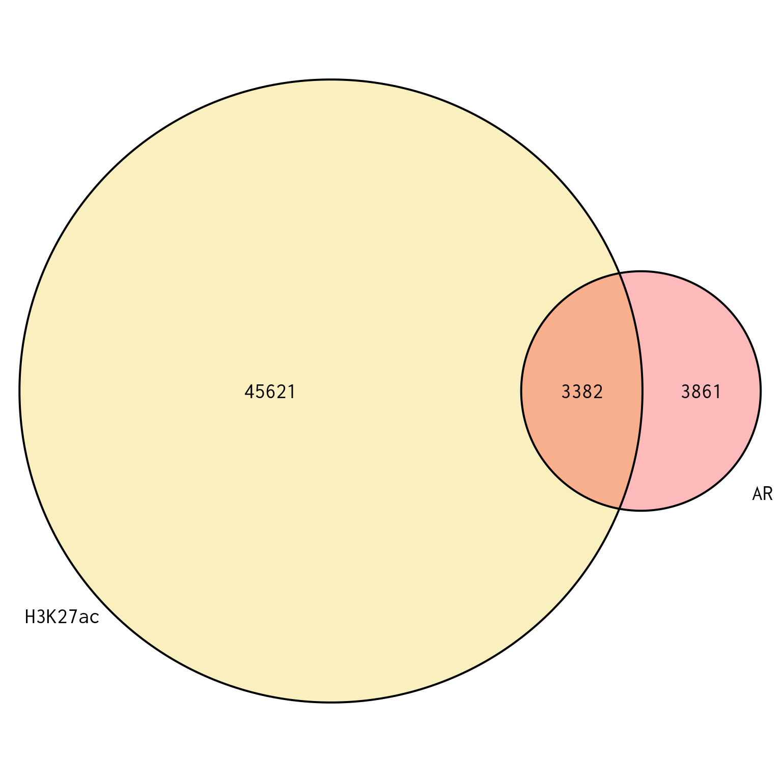
Union of peaks found in AR and H3K27ac, and which of the two targets each peak is found in. Peaks are based on the union of both sets of union peaks, which are themselves independent of treatment group.
Treatment Specific Peaks
size <- get_size_mode('exclusive_intersection')
yl <- "Set Size"
scale <- 1
if (max(vapply(treatment_peaks,length, integer(1))) > 1e4) {
  yl <- "Set Size ('000)"
  scale = 1e-3
}
treatment_peaks %>%
  .[rev(names(.))] %>%
  setNames(str_replace_all(names(.), "(.+)_(.+)", "\\1 (\\2)")) %>%
  plotOverlaps(
    .sort_sets = FALSE,
    set_col = treat_colours[vapply(., function(x) x$treat[[1]], character(1))],
    base_annotations = list(
      `Ranges in Intersection` = intersection_size(
        text_mapping = aes(label = comma(!!size)),
        bar_number_threshold = 1, text_colors = "black",
        text = list(size = 3.5, angle = 90, vjust = 0.5, hjust = -0.1)
      ) +
        scale_y_continuous(expand = expansion(c(0, 0.25)), label = comma) +
        theme(
          panel.grid = element_blank(),
          axis.line = element_line(colour = "grey20"),
          panel.border = element_rect(colour = "grey20", fill =  NA)
        )
    ),
    set_sizes = (
      upset_set_size() +
        geom_text(
          aes(label = comma(after_stat(count))),
          hjust = 1.1, stat = 'count', size = 3.5
        ) +
        scale_y_reverse(
          expand = expansion(c(0.3, 0)), label = comma_format(scale = scale)
        ) +
        ylab(yl) +
        theme(
          panel.grid = element_blank(),
          axis.line = element_line(colour = "grey20"),
          panel.border = element_rect(colour = "grey20", fill =  NA)
        )
    )
  ) +
  xlab("") +
  theme(
    text = element_text(size = 12),
    panel.grid = element_blank(),
    panel.border = element_rect(colour = "grey20", fill =  NA),
    axis.line = element_line(colour = "grey20")
  )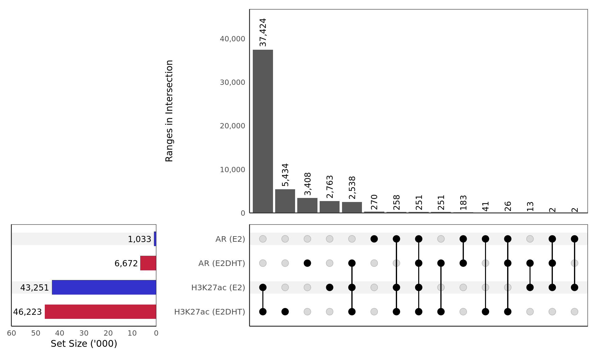
Macs2 peaks detected for AR and H3K27ac in the treatment groups E2 and E2DHT.
Differentially Bound Windows
cols <- c(cpm_column, "logFC", "status", fdr_column, "fdr_mu0", "centre")
lambda <- log2(config$comparisons$fc)
c1 <- comps[[1]]
c2 <- comps[[2]]
all_windows <- db_results %>%
  endoapply(mutate, centre = start + 0.5 * width) %>%
  mapGrlCols(var = cols) %>%
  mutate(
    distance = abs(!!sym(glue("{c1}_centre")) - !!sym(glue("{c2}_centre"))),
    "{c1}_status" := !!sym(glue("{c1}_status")) %>%
      fct_na_value_to_level("Undetected") %>%
      fct_relabel(\(x) paste(c1, x)),
    "{c2}_status" := !!sym(glue("{c2}_status")) %>%
      fct_na_value_to_level("Undetected") %>%
      fct_relabel(\(x) paste(c2, x)),
    status = case_when(
      ## Set everything where there's no unchanged values
      grepl("Up|Down|Undetected", !!sym(glue("{c1}_status"))) &
        grepl("Up|Down|Undetected", !!sym(glue("{c2}_status"))) ~ paste(
          !!sym(glue("{c1}_status")), !!sym(glue("{c2}_status")),
          sep = " - "
        ),
      ## Change status for comps[[2]] based on comps[[1]]
      grepl("Up|Down", !!sym(glue("{c1}_status"))) &
        !!sym(glue("{c2}_fdr_mu0")) >= fdr_alpha ~ paste(
          !!sym(glue("{c1}_status")), !!sym(glue("{c2}_status")),
          sep = " - "
        ),
      grepl("Up|Down", !!sym(glue("{c1}_status"))) &
        !!sym(glue("{c2}_logFC")) > lambda ~ paste0(
          !!sym(glue("{c1}_status")), glue(" - {c2} Up")
        ),
      grepl("Up|Down", !!sym(glue("{c1}_status"))) &
        !!sym(glue("{c2}_fdr_mu0")) < fdr_alpha &
        !!sym(glue("{c2}_logFC")) < -lambda ~ paste0(
          !!sym(glue("{c1}_status")), glue(" - {c2} Down")
        ),
      ## Change status for comps[[1]] based on comps[[2]]
      grepl("Up|Down", !!sym(glue("{c2}_status"))) &
        !!sym(glue("{c1}_fdr_mu0")) >= fdr_alpha ~ paste(
          !!sym(glue("{c1}_status")), !!sym(glue("{c2}_status")),
          sep = " - "
        ),
      grepl("Up|Down", !!sym(glue("{c2}_status"))) &
        !!sym(glue("{c1}_logFC")) > lambda ~ paste0(
          glue(" {c1} Up - "), !!sym(glue("{c2}_status"))
        ),
      grepl("Up|Down", !!sym(glue("{c2}_status"))) &
        !!sym(glue("{c1}_logFC")) < -lambda ~ paste0(
          glue(" {c1} Down - "), !!sym(glue("{c2}_status"))
        ),
      TRUE ~ paste(
          !!sym(glue("{c1}_status")), !!sym(glue("{c2}_status")),
          sep = " - "
        )
    ) %>%
      factor(levels = combs) %>%
      droplevels(),
    region = bestOverlap(., unlist(gene_regions), var = "region") %>%
      factor(levels = regions)
  )
## Remove any with an 'ambiguous' status
all_windows <- subset(all_windows, !is.na(status))
names(mcols(all_windows)) <- str_remove_all(
  names(mcols(all_windows)), "_ihw"
)
## Add features
if (has_features)
  all_windows$feature <- bestOverlap(
    all_windows, external_features, var = "feature", missing = "no_feature"
  ) %>%
  str_sep_to_title()

all_windows$hic <- NA
if (has_hic) all_windows$hic <- overlapsAny(all_windows, hic)

## Define promoters for mapping
feat_prom <- feat_enh <- GRanges()
if (has_features) {
  if ("feature" %in% colnames(mcols(external_features))) {
    feat_prom <- external_features %>%
      subset(str_detect(feature, "[Pp]rom")) %>%
      granges()
    feat_enh <- external_features %>%
      subset(str_detect(feature, "[Ee]nhanc")) %>%
      granges()
  }
}
prom4mapping <- c(feat_prom, granges(gene_regions$promoter)) %>%
  GenomicRanges::reduce()

all_windows <- all_windows %>%
  select(any_of(c("region", "feature", "hic")), everything()) %>%
  mapByFeature(
    gtf_gene, prom = prom4mapping, enh = feat_enh, gi = hic,
    gr2gene = extra_params$mapping$gr2gene,
    prom2gene = extra_params$mapping$prom2gene,
    enh2gene = extra_params$mapping$enh2gene, gi2gene = extra_params$mapping$gi2gene
  )
all_windows$detected <- all_windows$gene_name
if (has_rnaseq) all_windows$detected <- endoapply(
  all_windows$detected, intersect, rnaseq$gene_name
)
n_mapped <- all_windows %>%
  select(status, detected) %>%
  as_tibble() %>%
  unnest(everything()) %>%
  distinct(status, detected) %>%
  group_by(status) %>%
  summarise(mapped = dplyr::n()) %>%
  arrange(desc(mapped))
A set of 43,106 common windows was formed by obtaining the union of windows produced during the analysis of AR and H3K27ac individually. These common windows were formed using any overlap between target-specific windows. The window-to-gene mappings and the best overlap with genomic regions was also reformed. The best overlap with external features was also reformed.
In the original datasets, 13,512 windows were included for AR, whilst 33,900 windows were included for H3K27ac. The distance between each pair of windows was found by taking the centre of the original sliding window used for statistical analysis, and finding the difference. As windows were detected in an un-stranded manner, all distance values were set to be positive. Taking the complete set of 43,106 windows, 5,710 (13.2%) were considered as being detected in both datasets. The median distance between windows found in both comparisons was 400bp. 57 peaks (1.0%) were found to directly overlap.
Merged windows were compared across both targets and in order to obtain the best classification for each window, the initial values of an FDR-adjusted p-value < 0.05 from either comparison were used to consider a window as showing changed binding in at least one comparison. A secondary step was then introduced for each window such that if one target was significant and the other target had 1) received an FDR-adjusted p-value < 0.05 using a point-based \(H_0\), and 2) had an estimated logFC beyond the range specified for the range-based null hypothesis (\(H_0: 0 < |\mu| < \lambda\) for \(\lambda = 0.26\)), these windows were then considered significant in the second comparison. This was to help reduce the number of windows incorrectly classified as unchanged whilst the alternative ChIP target was defined as changed.
Whilst summary tables and figures are presented below, the full set of windows and mapped genes were exported as output/pairwise_comparisons/AR_H3K27ac/AR_E2_E2DHT-H3K27ac_E2_E2DHT-pairwise_comparison.csv.gz
cp <- htmltools::tags$em(
  glue(
    "Summary of combined binding windows for ",
    glue_collapse(comps, sep = " and "),
    ". Windows were classified as described above. ",
    "The number of windows showing each combined pattern are given, along ",
    "with the number of unique genes mapped to each set of combined windows, ",
    "noting that some genes will be mapped to multiple sets of windows. ",
    "The % of all genes with a window mapped from either target is given in ",
    "the final column."
  )
)
tbl <- all_windows %>%
  as_tibble() %>%
  rename_all(
    str_replace_all, pattern = "\\.Vs\\.\\.", replacement = " Vs. "
  ) %>%
  rename_all(
    str_replace_all, pattern = "\\.\\.", replacement = ": "
  ) %>%
  group_by(status) %>%
  summarise(
    windows = dplyr::n(),
    mapped = length(unique(unlist(gene_id))),
    .groups = "drop"
  ) %>%
  mutate(
    `% genes` = mapped / length(unique(unlist(all_windows$gene_id)))
  ) %>%
  separate(status, into = comps, sep = " - ") %>%
  reactable(
    filterable = TRUE,
    showPageSizeOptions = TRUE,
    columns = list2(
      !!sym(c1) := colDef(
        cell = function(value) {
          value <- str_extract(value, "Up|Down|Unchanged|Undetected")
          if (str_detect(value, "Up")) value <- paste(value, "\u21E7")
          if (str_detect(value, "Down")) value <- paste(value, "\u21E9")
          paste(targets[[1]], value)
        },
        style = function(value) {
          colour <- case_when(
            str_detect(value, "Up") ~ colours$direction[["up"]],
            str_detect(value, "Down") ~ colours$direction[["down"]],
            str_detect(value, "Unchanged") ~ colours$direction[["unchanged"]],
            str_detect(value, "Undetected") ~ colours$direction[["undetected"]]
          )
          list(color = colour)
        },
        footer = htmltools::tags$b("Total")
      ),
      !!sym(c2) := colDef(
        cell = function(value) {
          value <- str_extract(value, "Up|Down|Unchanged|Undetected")
          if (str_detect(value, "Up")) value <- paste(value, "\u21E7")
          if (str_detect(value, "Down")) value <- paste(value, "\u21E9")
          paste(targets[[2]], value)
        },
        style = function(value) {
          colour <- case_when(
            str_detect(value, "Up") ~ colours$direction[["up"]],
            str_detect(value, "Down") ~ colours$direction[["down"]],
            str_detect(value, "Unchanged") ~ colours$direction[["unchanged"]],
            str_detect(value, "Undetected") ~ colours$direction[["undetected"]]
          )
          list(color = colour)
        }
      ),
      windows = colDef(
        name = "Number of Windows",
        cell = function(value) comma(value, 1),
        style = function(value) {
          bar_style(width = 0.9*value / length(all_windows), fill = "#B3B3B3")
        },
        footer = htmltools::tags$b(comma(length(all_windows), 1))
      ),
      mapped = colDef(
        name = "Mapped Genes",
        cell = function(value) comma(value, 1),
        style = function(value) {
          bar_style(width = 0.9*value / length(unique(unlist(all_windows$gene_id))), fill = "#B3B3B3")
        },
        footer = htmltools::tags$b(comma(length(unique(unlist(all_windows$gene_id))), 1))
      ),
      `% genes` = colDef(
        name = "% Of All Mapped Genes",
        cell = function(x) percent(x, 0.1),
        style = function(value) {
          bar_style(width = 0.9*value, fill = "#B3B3B3")
        }
      )
    )
  )
div(class = "table",
    div(class = "table-header",
        div(class = "caption", cp),
        tbl
    )
)Pairwise Differential Binding
df <- all_windows %>%
  select(ends_with("logFC"), status, detected, any_of(c("region", "feature"))) %>%
  as_tibble()
x_range <- range(df[[glue("{c1}_logFC")]], na.rm = TRUE)
y_range <- range(df[[glue("{c2}_logFC")]], na.rm = TRUE)
df %>%
  mutate(status = fct_lump_min(status, 2)) %>%
  ggplot() +
  geom_ysideboxplot(
    aes(status, !!sym(glue("{c2}_logFC")), fill = status),
    orientation = "x",
    data = df %>%
      dplyr::filter(!grepl(paste(c2, "Undetected"), status)) %>%
      mutate(status = str_remove_all(status, " - .+"))
  ) +
  geom_xsideboxplot(
    aes(!!sym(glue("{c1}_logFC")), status, fill = status),
    orientation = "y",
    data = df %>%
      dplyr::filter(!grepl(paste(c1, "Undetected"), status)) %>%
      mutate(status = str_remove_all(status, ".+ - "))
  ) +
  geom_point(
    aes(!!sym(glue("{c1}_logFC")), !!sym(glue("{c2}_logFC")), colour = status),
    data = . %>% dplyr::filter(!grepl("Undetected", status)),
    alpha = 0.6
  ) +
  geom_hline(yintercept = 0) +
  geom_hline(
    yintercept = c(1, -1) * lambda,
    linetype = 2, colour = "grey"
  ) +
  geom_vline(xintercept = 0) +
  geom_vline(
    xintercept = c(1, -1) * lambda,
    linetype = 2, colour = "grey"
  ) +
  geom_label_repel(
    aes(
      !!sym(glue("{c1}_logFC")), !!sym(glue("{c2}_logFC")), colour = status,
      label = label
    ),
    data = . %>%
      dplyr::filter(!grepl("Undetected|Other", status)) %>%
      dplyr::filter(!grepl("Un.+Un", status)) %>%
      mutate(d = .[[glue("{c1}_logFC")]]^2 + .[[glue("{c2}_logFC")]]^2) %>%
      dplyr::filter(vapply(detected, length, integer(1)) > 0) %>%
      dplyr::filter(d == max(d), d > 1, .by = status) %>%
      mutate(
        label = vapply(detected, paste, character(1), collapse = "; ") %>%
          str_wrap(25)
      ),
    force_pull = 1/10, force = 10,
    min.segment.length = 0.05,
    size = 4, fill = rgb(1, 1, 1, 0.4),
    show.legend = FALSE
  ) +
  annotate(
    "text",
    x = 0.95 * diff(x_range) + min(x_range),
    y = 0.05 * diff(y_range) + min(y_range),
    label = paste("n =", comma(sum(!grepl("Undetected", df$status))))
  ) +
  annotate(
    "text",
    x = 0.05 * diff(x_range) + min(x_range),
    y = 0.95 * diff(y_range) + min(y_range),
    label = paste(
      "rho == ",
      cor(
        df[[glue("{c1}_logFC")]], df[[glue("{c2}_logFC")]],
        use = "pairwise.complete.obs"
      ) %>%
        round(3)
    ),
    parse = TRUE
  ) +
  scale_xsidey_discrete(position = "right") +
  scale_ysidex_discrete(label = label_wrap(30)) +
  scale_x_continuous() +
  scale_colour_manual(values = group_colours, labels = label_wrap(20)) +
  scale_fill_manual(
    values = comps %>%
      lapply(function(x){
        cols <- unlist(colours$direction)
        names(cols) <- paste(x, str_to_title(names(cols)))
        cols
      }) %>%
      unlist()
  ) +
  labs(
    x = paste(c1, "logFC"), y = paste(c2, "logFC"), colour = "Status"
  ) +
  guides(fill = "none") +
  theme(
    ggside.panel.scale.y = .2, ggside.panel.scale.x = .3,
    ggside.axis.text.x.bottom = element_text(angle = 90, hjust = 1, vjust = 0.5),
    axis.title.x = element_text(hjust = 0.52 * (1 - 0.2), vjust = 18),
    axis.title.y = element_text(hjust = 0.52 * (1 - 0.3)),
    legend.key.height = unit(0.075, "npc")
  )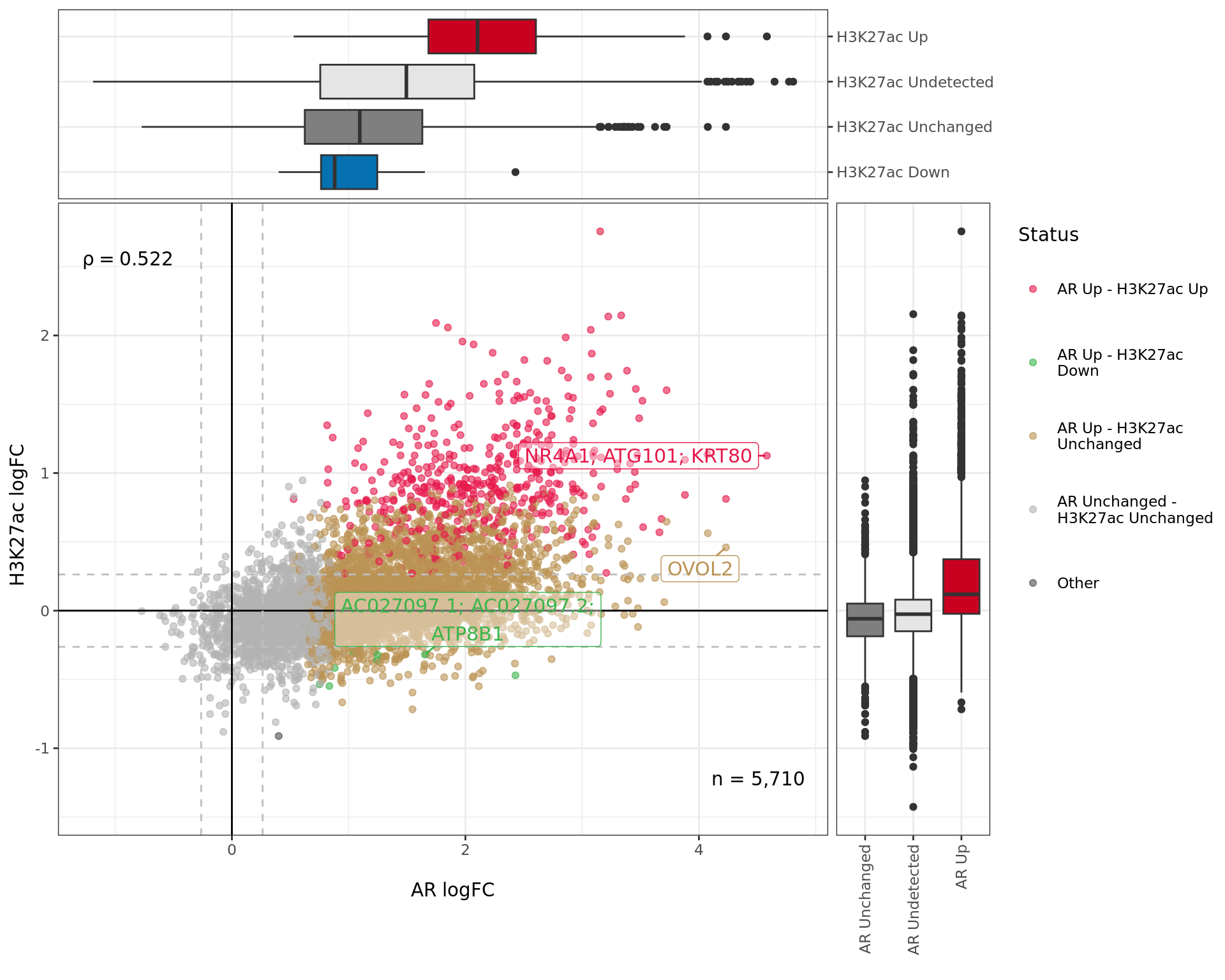
Comparative changes in both AR and H3K27ac. The window with most extreme combined change in binding is shown with any mapped genes labelled. The range around zero used for range-based hypothesis testing is indicated with grey dashed lines.
logFC By Region
df %>%
  mutate(status = fct_lump_min(status, 2)) %>%
  ggplot() +
  geom_point(
    aes(!!sym(glue("{c1}_logFC")), !!sym(glue("{c2}_logFC")), colour = status),
    data = . %>% dplyr::filter(!grepl("Undetected", status)),
    alpha = 0.6
  ) +
  geom_hline(yintercept = 0) +
  geom_hline(
    yintercept = c(1, -1) * lambda,
    linetype = 2, colour = "grey"
  ) +
  geom_vline(xintercept = 0) +
  geom_vline(
    xintercept = c(1, -1) * lambda,
    linetype = 2, colour = "grey"
  ) +
  geom_label_repel(
    aes(
      !!sym(glue("{c1}_logFC")), !!sym(glue("{c2}_logFC")), colour = status,
      label = label
    ),
    data = . %>%
      dplyr::filter(!grepl("Undetected|Other", status)) %>%
      dplyr::filter(!grepl("Un.+Un", status)) %>%
      mutate(d = .[[glue("{c1}_logFC")]]^2 + .[[glue("{c2}_logFC")]]^2) %>%
      dplyr::filter(vapply(detected, length, integer(1)) > 0) %>%
      dplyr::filter(d == max(d), .by = c(status,region)) %>%
      dplyr::filter(d > 1) %>%
      mutate(
        label = vapply(detected, paste, character(1), collapse = "; ") %>%
          str_wrap(20) %>%
          str_trunc(35)
      ),
    force_pull = 1/10, force = 10,
    min.segment.length = 0.05,
    size = 3.5, fill = rgb(1, 1, 1, 0.4),
    show.legend = FALSE
  ) +
  geom_text(
    aes(x, y, label = label),
    data = . %>%
      dplyr::filter(!grepl("Undetected", status)) %>%
      summarise(n = dplyr::n(), .by = region) %>%
      mutate(
        x = min(x_range) + 0.9 * diff(x_range),
        y = min(y_range) + 0.05 * diff(y_range),
        label = paste("n =", comma(n, 1))
      )
  ) +
  facet_wrap(~region) +
  scale_colour_manual(values = group_colours, labels = label_wrap(20)) +
  scale_fill_manual(
    values = comps %>%
      lapply(function(x){
        cols <- unlist(colours$direction)
        names(cols) <- paste(x, str_to_title(names(cols)))
        cols
      }) %>%
      unlist()
  ) +
  labs(
    x = paste(c1, "logFC"), y = paste(c2, "logFC"), colour = "Status"
  ) +
  guides(fill = "none") +
  theme(
    ggside.panel.scale.y = .2, ggside.panel.scale.x = .3,
    ggside.axis.text.x.bottom = element_text(angle = 90, hjust = 1, vjust = 0.5),
    legend.key.height = unit(0.075, "npc")
  )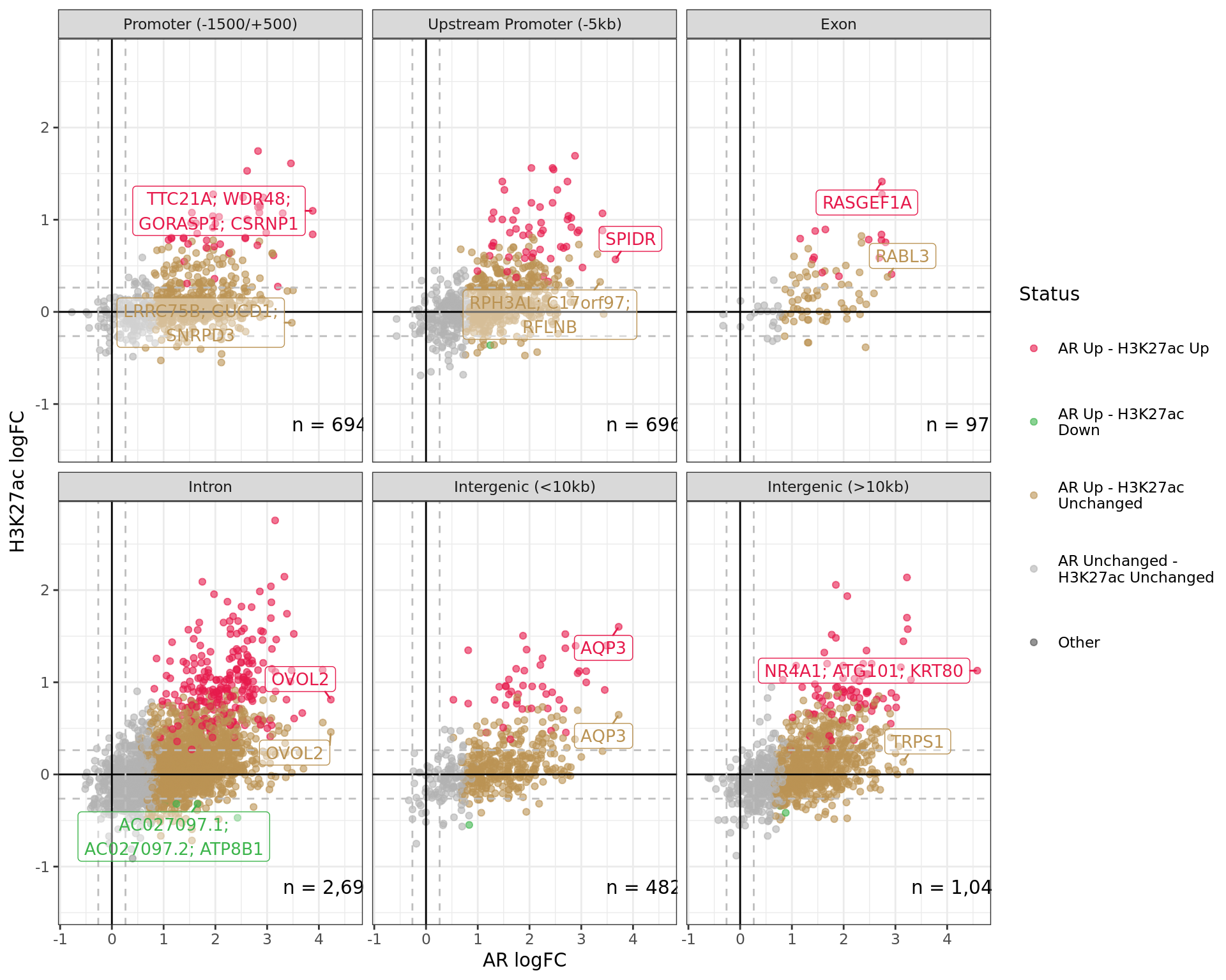
Comparative changes in both AR and H3K27ac. The window with most extreme combined change in binding for each separate region is shown with any mapped genes labelled. The range around zero used for range-based hypothesis testing is indicated with grey dashed lines.
logFC By Feature
df %>%
  mutate(status = fct_lump_min(status, 2)) %>%
  ggplot() +
  geom_point(
    aes(!!sym(glue("{c1}_logFC")), !!sym(glue("{c2}_logFC")), colour = status),
    data = . %>% dplyr::filter(!grepl("Undetected", status)),
    alpha = 0.6
  ) +
  geom_hline(yintercept = 0) +
  geom_hline(
    yintercept = c(1, -1) * lambda,
    linetype = 2, colour = "grey"
  ) +
  geom_vline(xintercept = 0) +
  geom_vline(
    xintercept = c(1, -1) * lambda,
    linetype = 2, colour = "grey"
  ) +
  geom_label_repel(
    aes(
      !!sym(glue("{c1}_logFC")), !!sym(glue("{c2}_logFC")), colour = status,
      label = label
    ),
    data = . %>%
      dplyr::filter(!grepl("Undetected|Other", status)) %>%
      dplyr::filter(!grepl("Un.+Un", status)) %>%
      mutate(d = .[[glue("{c1}_logFC")]]^2 + .[[glue("{c2}_logFC")]]^2) %>%
      dplyr::filter(vapply(detected, length, integer(1)) > 0) %>%
      dplyr::filter(d == max(d), .by = c(status, feature)) %>%
      dplyr::filter(d > 1) %>%
      mutate(
        label = vapply(detected, paste, character(1), collapse = "; ") %>%
          str_wrap(20) %>%
          str_trunc(35)
      ),
    force_pull = 1/10, force = 10,
    min.segment.length = 0.05,
    size = 3.5, fill = rgb(1, 1, 1, 0.4),
    show.legend = FALSE
  ) +
  geom_text(
    aes(x, y, label = label),
    data = . %>%
      dplyr::filter(!grepl("Undetected", status)) %>%
      summarise(n = dplyr::n(), .by = feature) %>%
      mutate(
        x = min(x_range) + 0.9 * diff(x_range),
        y = min(y_range) + 0.05 * diff(y_range),
        label = paste("n =", comma(n, 1))
      )
  ) +
  facet_wrap(~feature) +
  scale_colour_manual(values = group_colours, labels = label_wrap(20)) +
  scale_fill_manual(
    values = comps %>%
      lapply(function(x){
        cols <- unlist(colours$direction)
        names(cols) <- paste(x, str_to_title(names(cols)))
        cols
      }) %>%
      unlist()
  ) +
  labs(
    x = paste(c1, "logFC"), y = paste(c2, "logFC"), colour = "Status"
  ) +
  guides(fill = "none") +
  theme(
    ggside.panel.scale.y = .2, ggside.panel.scale.x = .3,
    ggside.axis.text.x.bottom = element_text(angle = 90, hjust = 1, vjust = 0.5),
    legend.key.height = unit(0.075, "npc")
  )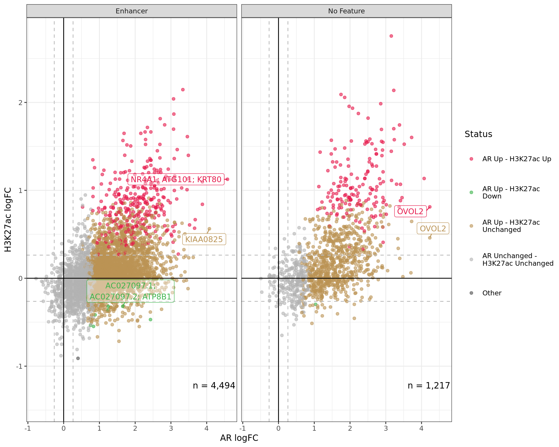
Comparative changes in both AR and H3K27ac. The window with most extreme combined change in binding for each separate feature is shown with any mapped genes labelled. The range around zero used for range-based hypothesis testing is indicated with grey dashed lines.
Pairwise Signal
db_results %>%
  plotPairwise(
    var = cpm_column, alpha = 0.6, side_panel_width = 0.2,
  ) +
  scale_fill_manual(
    values = setNames(
      comp_cols, paste(names(comp_cols), c("Only", "Only", "Detected"))
    )
  )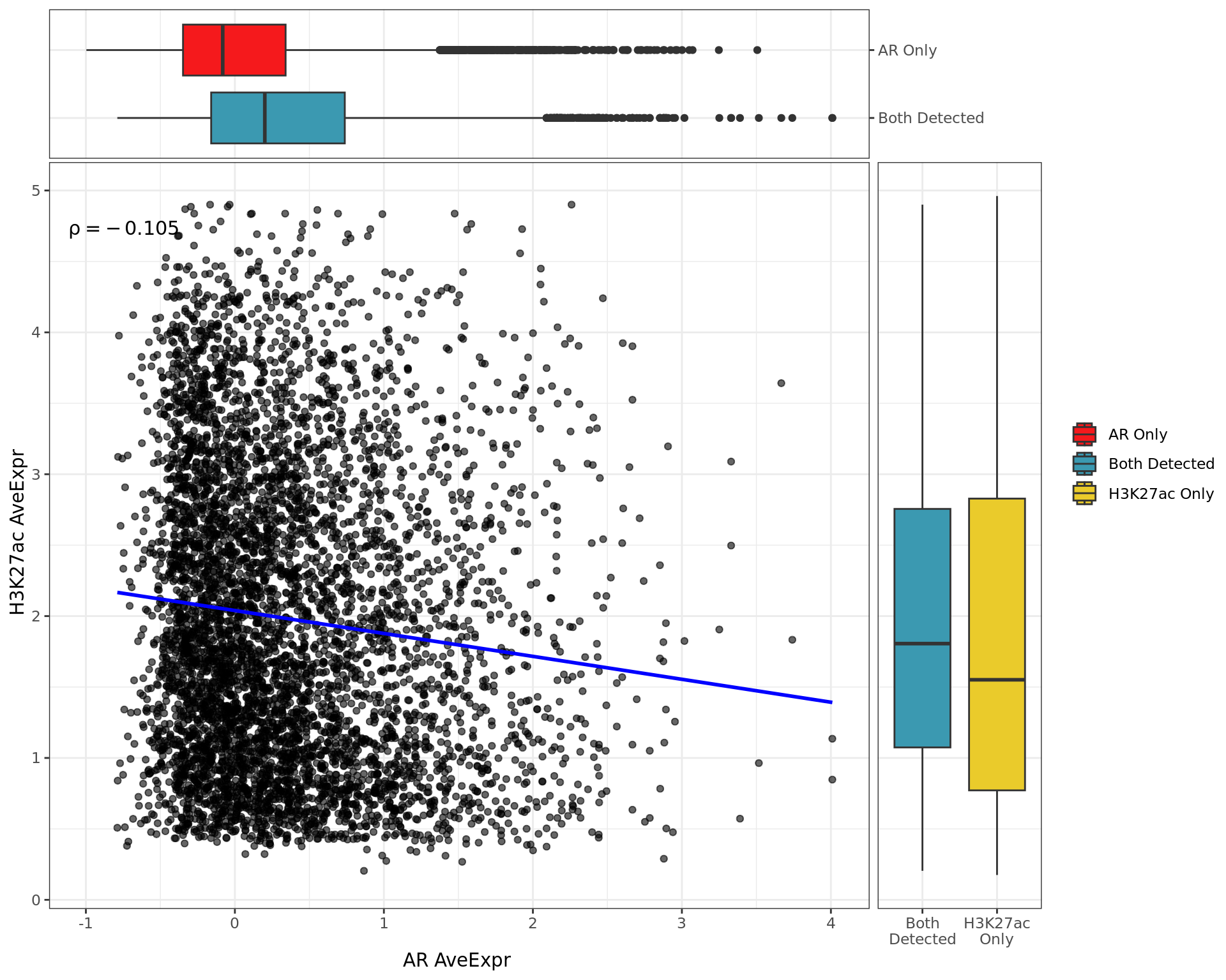
Pairwise signal levels with boxplots indicating the baseline signal whether signal was detected in both or individual comparisons.
Distribution By Region
all_windows %>%
  filter(grepl("Up|Down", status)) %>%
  mutate(status = fct_lump_prop(status, 0.01)) %>%
  plotSplitDonut(
    outer = "region",
    inner = "status",
    inner_palette = group_colours,
    outer_palette = region_colours,
    inner_glue = "{str_replace_all(.data[[inner]], ' - ', '\n')}\nn = {comma(n, 1)}\n{percent(p,0.1)}",
    outer_glue = "{str_wrap(.data[[outer]], 15)}\nn = {comma(n, 1)}\n{percent(p,0.1)}",
    outer_min_p = 0.025, inner_label_alpha = 0.8,
    explode_inner = "(Up|Down).+(Up|Down)", explode_r = 1/3
  )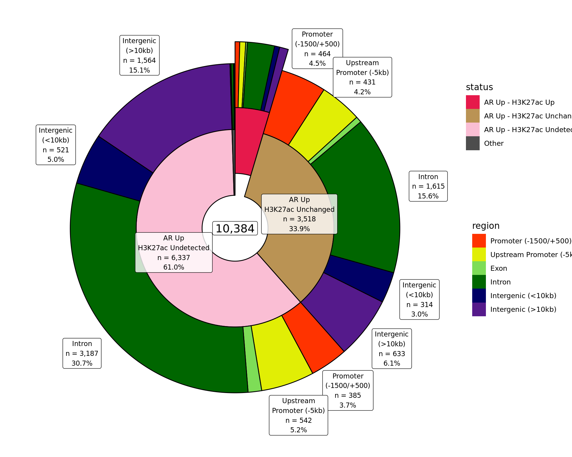
Distribution of binding patterns by genomic regions as defined in earlier sections. Windows are only shown if change was detected in one of the comparisons. Segments where changes were detected in both comparisons are exploded.
Distribution By Feature
all_windows %>%
  filter(grepl("Up|Down", status)) %>%
  mutate(status = fct_lump_prop(status, 0.01)) %>%
  plotSplitDonut(
    outer = "feature",
    inner = "status",
    inner_palette = group_colours,
    outer_palette = feature_colours,
    inner_glue = "{str_replace_all(.data[[inner]], ' - ', '\n')}\nn = {comma(n, 1)}\n{percent(p,0.1)}",
    outer_glue = "{str_wrap(.data[[outer]], 15)}\nn = {comma(n, 1)}\n{percent(p,0.1)}",
    outer_min_p = 0.025, inner_label_alpha = 0.8,
    explode_inner = "(Up|Down).+(Up|Down)", explode_r = 1/3
  )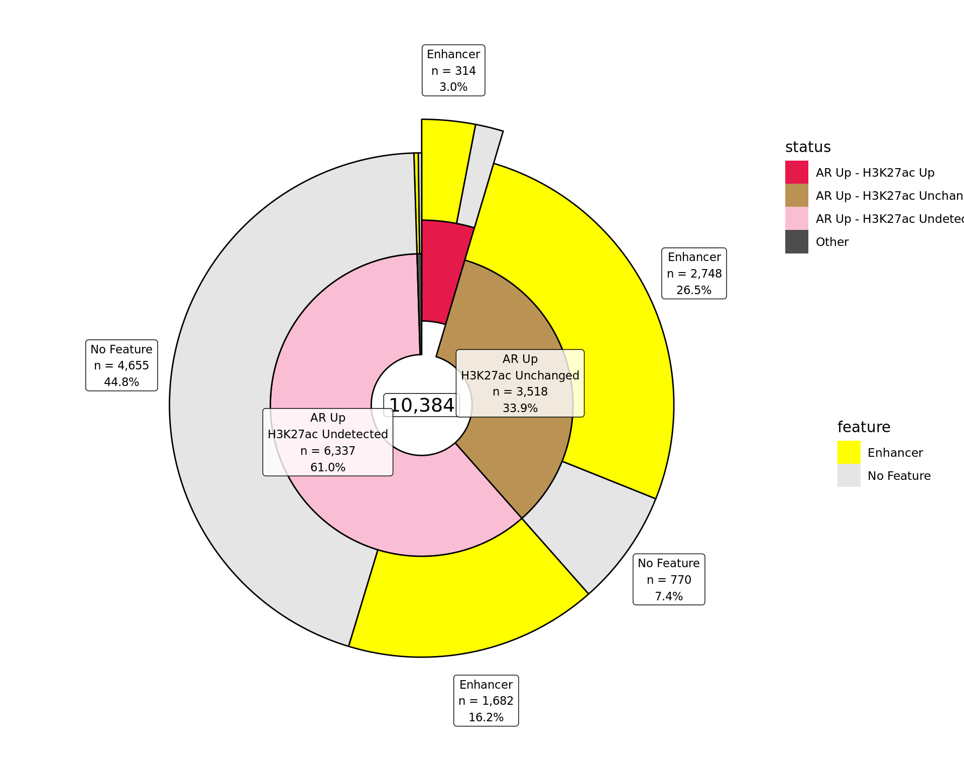
Distribution of binding patterns by external features as defined in earlier sections. Windows are only shown if change was detected in one of the comparisons.
Distance By Status
all_windows %>%
  as_tibble() %>%
  dplyr::filter(!is.na(distance)) %>%
  arrange(status, distance) %>%
  group_by(status) %>%
  mutate(
    n = dplyr::n(),
    q = seq_along(status) / n
  ) %>%
  dplyr::filter(distance < 1e3, str_detect(status, "Up|Down"), n > 10) %>%
  ggplot(aes(distance, q, colour = status)) +
  geom_line(linewidth = 1) +
  scale_x_continuous(breaks = seq(0, 10, by = 2) * 100) +
  scale_y_continuous(
    labels = percent, expand = expansion(c(0, 0.05)),
    breaks = seq(0, 1, by = 0.2)
  ) +
  scale_colour_manual(
    values = group_colours
  ) +
  labs(
    x = "Distance Between Window Centres (bp)",
    y = "Percentile",
    colour = "Combined Status"
  )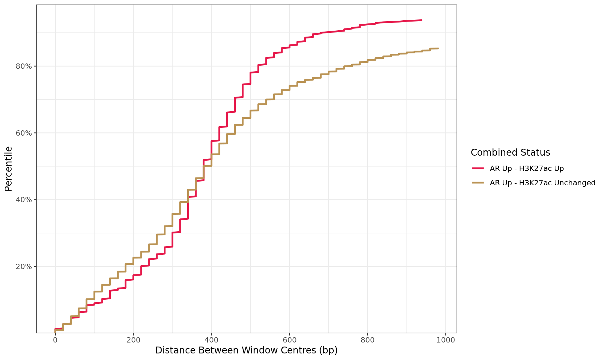
Distances between windows where maximal signal was detected for each target. Windows are only shown if change was detected in one or more comparisons, and if 10 or more windows were found in each group. The x-axis is truncated at 1kb
Distance by Region
all_windows %>%
  as_tibble() %>%
  dplyr::filter(!is.na(distance)) %>%
  arrange(region, distance) %>%
  group_by(region) %>%
  mutate(
    n = dplyr::n(),
    q = seq_along(region) / n
  ) %>%
  dplyr::filter(distance < 1e3) %>%
  ggplot(aes(distance, q, colour = region)) +
  geom_line(linewidth = 1) +
  scale_x_continuous(breaks = seq(0, 10, by = 2) * 100) +
  scale_y_continuous(
    labels = percent, expand = expansion(c(0, 0.05)),
    breaks = seq(0, 1, by = 0.2)
  ) +
  scale_colour_manual(values = region_colours) +
  labs(
    x = "Distance Between Window Centres (bp)",
    y = "Percentile",
    colour = "Genomic Region"
  )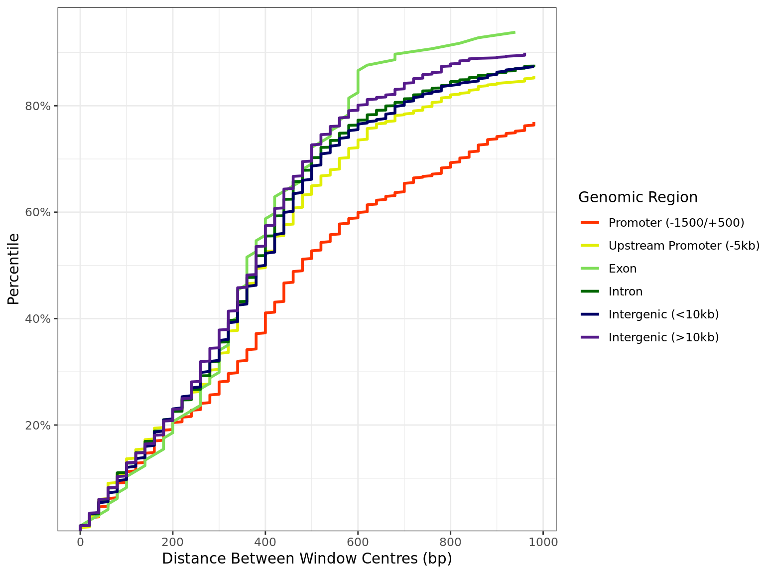
Distribution of distances between peaks separated by genomic region. All sites are included regardless of changed binding. The x-axis is truncated 1kb.
Distance By Feature
all_windows %>%
  as_tibble() %>%
  dplyr::filter(!is.na(distance)) %>%
  mutate(feature = factor(feature, levels = names(feature_colours))) %>%
  arrange(feature, distance) %>%
  group_by(feature) %>%
  mutate(
    n = dplyr::n(),
    q = seq_along(feature) / n
  ) %>%
  dplyr::filter(distance < 1e3) %>%
  droplevels() %>%
  ggplot(aes(distance, q, colour = feature)) +
  geom_line(linewidth = 1) +
  scale_x_continuous(breaks = seq(0, 10, by = 2) * 100) +
  scale_y_continuous(
    labels = percent, expand = expansion(c(0, 0.05)),
    breaks = seq(0, 1, by = 0.2)
  ) +
  scale_colour_manual(values = unlist(feature_colours)) +
  labs(
    x = "Distance Between Window Centres (bp)",
    y = "Percentile",
    colour = "External Feature"
  )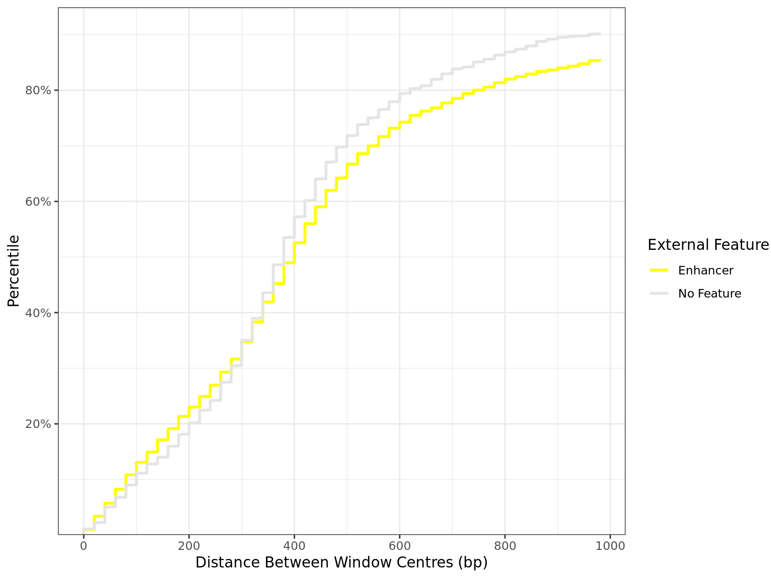
Distribution of distances between peaks separated by external feature. All sites are included regardless of changed binding. The x-axis is truncated 1kb.
Combined Binding
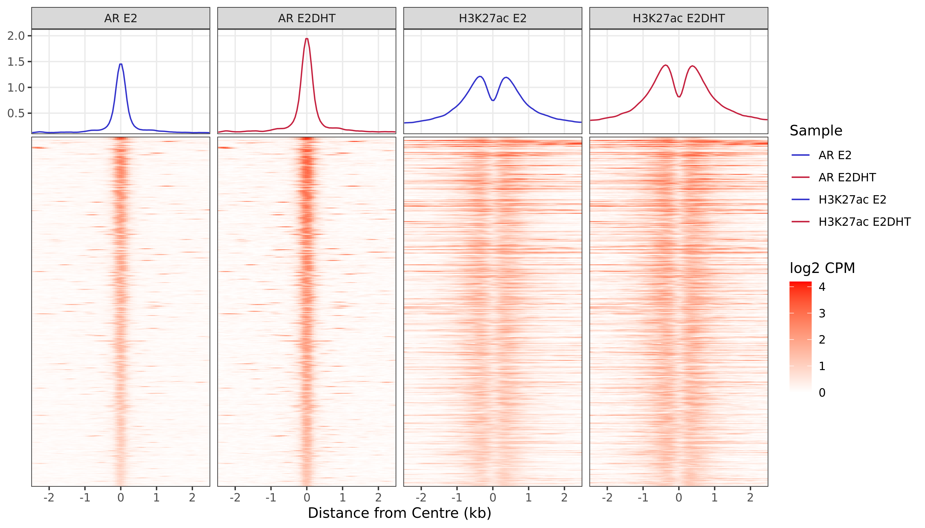
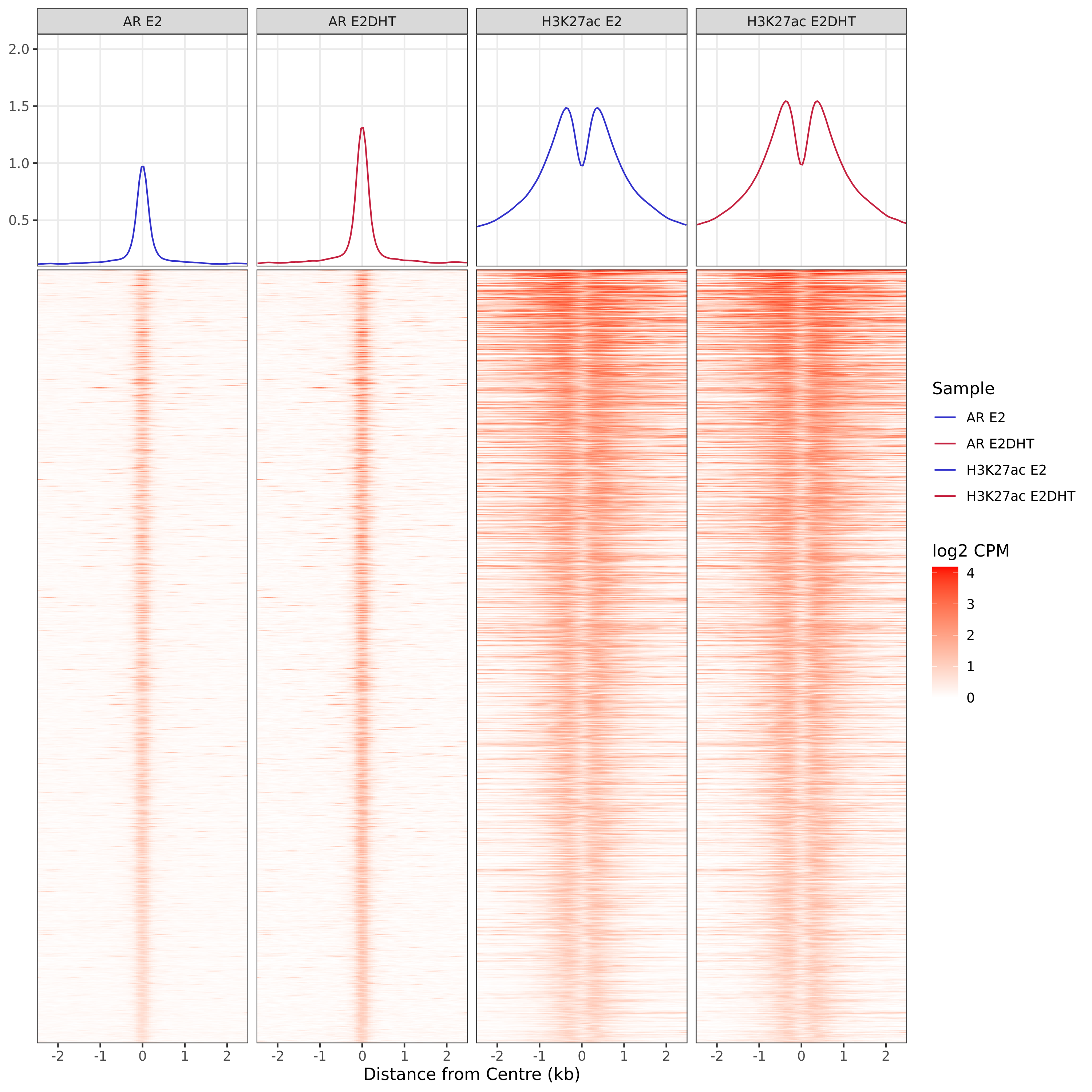
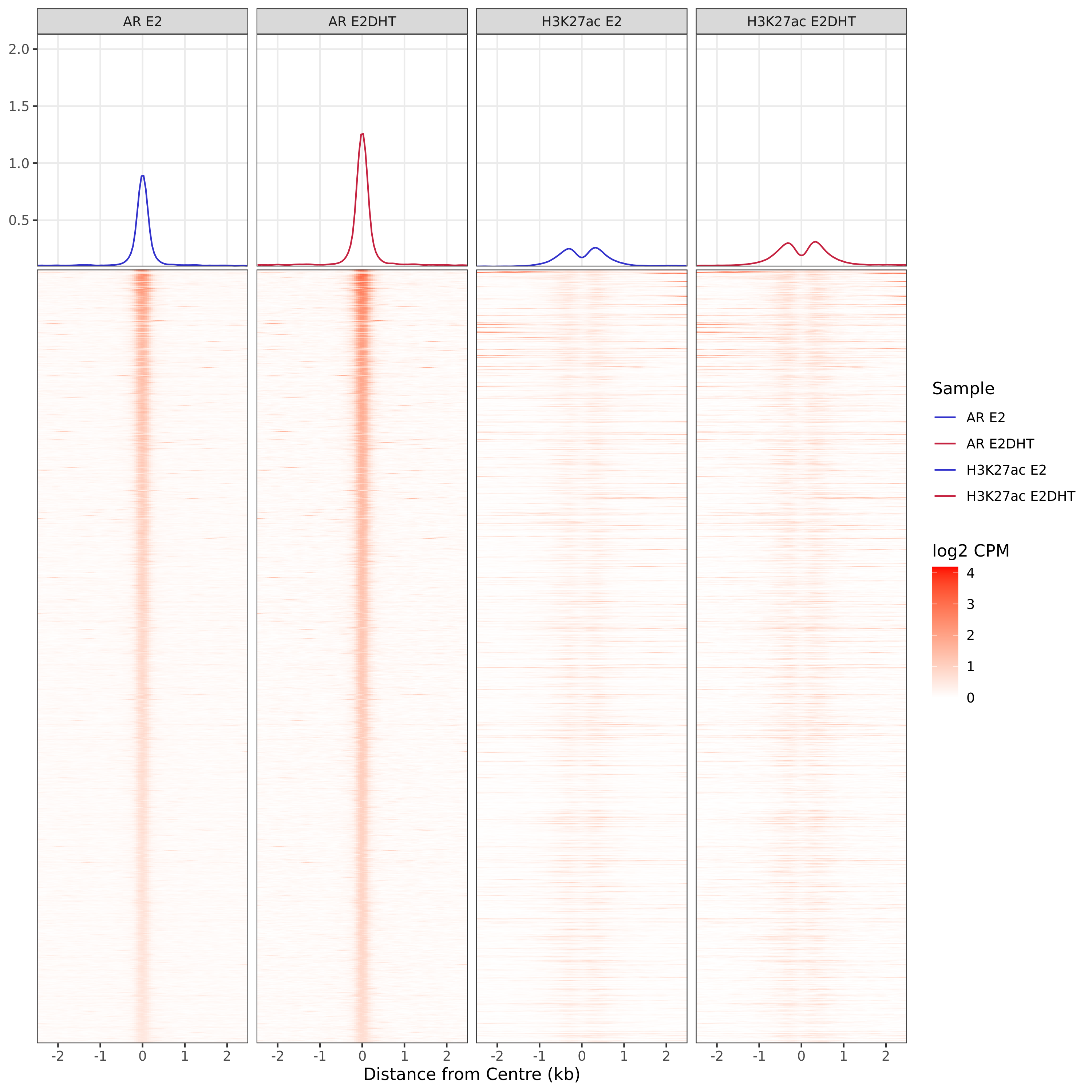
Heatmaps
A series of profile heatmaps were generated for any set of pairwise comparisons with more than 25 ranges, and where binding was detected as changed in at least one of the comparisons. If comparing two targets, peaks were centred at the mid-point between the ranges of individual maximal signal. If only one target is detected within a range, peaks are centred at the range with maximal signal. Scales for fill and average signal (both logCPM) are held constant across all plots for easier comparison between groups.
## Set the BWFL as a single object incorporating target & treatment names
fl <- seq_along(pairs) %>%
  lapply(
    function(x) {
      file.path(
        macs2_path[[x]],
         # glue("{names(pairs)[x]}_{pairs[[x]]}_merged_FE.bw")
         glue("{names(pairs)[x]}_{pairs[[x]]}_merged_treat_pileup.bw")
      ) %>%
        setNames(paste(names(pairs)[[x]], pairs[[x]]))
    }
  ) %>%
  unlist() %>%
  .[!duplicated(.)]
bwfl_fe <- setNames(BigWigFileList(fl), names(fl))
n_bins <- 100
n_max <- 2000
grl_to_plot <- all_windows %>%
  split(.$status) %>%
  .[str_detect(names(.),"Up|Down")] %>%
  .[vapply(., length, integer(1)) > 25] %>% # Only show groups with > 25 ranges
  lapply(
    mutate,
    centre = case_when(
      is.na(!!sym(glue("{c1}_centre"))) ~ !!sym(glue("{c2}_centre")),
      !is.na(!!sym(glue("{c1}_centre"))) ~ !!sym(glue("{c1}_centre"))
    ),
    rng = paste0(seqnames, ":", as.integer(centre))
  ) %>%
  lapply(function(x) GRanges(x$rng, seqinfo = sq)) %>%
  GRangesList() %>%
  endoapply(distinctMC)
profile_width <- 5e3
x_lab <- c(
  seq(0, floor(0.5 * profile_width / 1e3), length.out = 3),
  seq(-floor(0.5 * profile_width / 1e3), 0, length.out = 3)
) %>%
  sort() %>%
  unique()
sig_profiles <- grl_to_plot %>%
  endoapply(
    function(x) {
      if (length(x) <= n_max) return(x)
      id <- sample(length(x), n_max)
      sort(x[id])
    }
  ) %>%
  mclapply(
    function(x) getProfileData(
      bwfl_fe, x, upstream = profile_width / 2, bins = n_bins, log = TRUE
    ),
    mc.cores = min(length(grl_to_plot), threads)
  )
profile_heatmaps <- sig_profiles %>%
  mclapply(
    plotProfileHeatmap,
    profileCol = "profile_data",
    xLab = "Distance from Centre (bp)",
    fillLab = "log2 CPM",
    colour = "name",
    mc.cores = min(length(.), threads)
  )
fill_range <- profile_heatmaps %>%
  lapply(function(x) x$data[,"score"]) %>%
  unlist() %>%
  c(0) %>%
  range()
sidey_range <- profile_heatmaps %>%
  lapply(function(x) x$layers[[3]]$data$y) %>%
  unlist() %>%
  range()
profile_heatmaps <- profile_heatmaps %>%
  lapply(
    function(x) {
      x +
        scale_x_continuous(
          breaks = x_lab * 1e3, labels = x_lab, expand = expansion(0)
        ) +
        scale_xsidey_continuous(
          limits = sidey_range, expand = expansion(c(0, 0.1))
        ) +
        scale_fill_gradientn(colours = colours$heatmaps, limits = fill_range) +
        scale_colour_manual(
          values = lapply(
            seq_along(pairs),
            function(i) setNames(
              treat_colours[pairs[[i]]],
              paste(names(pairs)[[i]], pairs[[i]])
            )
          ) %>%
            unlist() %>%
            .[!duplicated(names(.))]
        ) +
        labs(
          x = "Distance from Centre (kb)",
          fill = "log2 CPM", linetype = "Union\nPeak\nOverlap",
          colour = "Sample"
        )
    }
  )
htmltools::tagList(
mclapply(
seq_along(profile_heatmaps),
function(x) {
## Export the image
pw <- names(profile_heatmaps)[[x]]
img_out <- file.path(
fig_path,
pw %>%
str_remove_all("(:|Vs. |- )") %>%
str_replace_all(" ", "_") %>%
str_replace_all("_-_", "-") %>%
paste0("_profile_heatmap.", fig_type)
)
n_ranges <- length(grl_to_plot[[x]])
n_samples <- length(unique(profile_heatmaps[[x]]$data$name))
fig_fun(
filename = img_out,
width = knitr::opts_current$get("fig.width") * n_samples / 4,
height = min(
3.5 + knitr::opts_current$get("fig.height") * n_ranges / 1.5e3,
10
)
)
print(profile_heatmaps[[x]])
dev.off()
## Create html tags
fig_link <- str_extract(img_out, "assets.+")
cp <- htmltools::tags$em(
glue(
"
{n_ranges} ranges were defined as showing the pattern {pw}. Ranges were
centered at the midpoint between ranges identified as the maximal
signal range, based on {c1} only. If more than {n_max} ranges were
defined, plots were restricted to {n_max} ranges. Values showb are log2
CPM taking the SPMR-based bigwig files produced by macs callpeak.
"
)
)
htmltools::div(
htmltools::div(
id = img_out %>%
basename() %>%
str_remove_all(glue(".{fig_type}$")) %>%
str_to_lower() %>%
str_replace_all("_", "-"),
class = "section level3",
htmltools::h3(pw),
htmltools::div(
class = "figure", style = "text-align: center",
htmltools::img(src = fig_link, width = "100%"),
htmltools::tags$caption(cp)
)
)
)
},
mc.cores = threads
)
)AR Up - H3K27ac Up
AR Up - H3K27ac Unchanged
AR Up - H3K27ac Undetected
Windows With The Strongest Signal
For the initial set of visualisations, the sets of windows with the strongest signal were selected from within each group. Groups were restricted to those where differential binding was seen in at least comparison.
grl_to_plot <- all_windows %>%
  filter(
    !str_detect(status, "Un.+Un"),
    vapply(detected, length, integer(1)) > 0
  ) %>%
  as_tibble() %>%
  rename_all(
    str_replace_all, pattern = "\\.Vs\\.\\.", replacement = " Vs. "
  ) %>%
  rename_all(
    str_replace_all, pattern = "\\.\\.", replacement = ": "
  ) %>%
  nest(
    AveExpr = ends_with("AveExpr")
  ) %>%
  mutate(
    max_signal = vapply(AveExpr, function(x) max(unlist(x)), numeric(1))
  ) %>%
  group_by(status) %>%
  filter(max_signal == max(max_signal)) %>%
  dplyr::select(
    range, status, ends_with("logFC")
  ) %>%
  droplevels() %>%
  split(.$status) %>%
  lapply(pull, "range") %>%
  lapply(function(x) x[1]) %>%
  lapply(GRanges, seqinfo = sq) %>%
  GRangesList()
## The coverage
bwfl <- seq_along(pairs) %>%
lapply(
function(x) {
file.path(
macs2_path[[x]],
glue("{names(pairs)[x]}_{pairs[[x]]}_merged_treat_pileup.bw")
) %>%
BigWigFileList() %>%
setNames(pairs[[x]])
}
) %>%
setNames(comps)
line_col <- lapply(bwfl, function(x) treat_colours[names(x)])
## Coverage annotations
annot <- comps %>%
lapply(
function(x) {
col <- glue("{x}_status")
select(all_windows, all_of(col)) %>%
mutate(
status = str_extract(!!sym(col), "Down|Up|Unchanged|Undetected")
) %>%
splitAsList(.$status) %>%
lapply(granges) %>%
lapply(unique) %>%
GRangesList()
}
) %>%
setNames(comps)
annot_col <- unlist(colours$direction) %>%
setNames(str_to_title(names(.)))
## Coverage y-limits
gr <- unlist(grl_to_plot)
y_lim <- lapply(
bwfl,
function(x) {
cov <- lapply(x, import.bw, which = gr)
unlist(lapply(cov, function(y) max(y$score))) %>%
c(0) %>%
range()
}
)
## The features track
feat_gr <- gene_regions %>%
lapply(granges) %>%
GRangesList()
feature_colours <- colours$regions
if (has_features) {
feat_gr <- list(Regions = feat_gr)
feat_gr$Features <- splitAsList(external_features, external_features$feature)
feature_colours <- list(
Regions = unlist(colours$regions),
Features = unlist(colours$features)
)
}
## The genes track
hfgc_genes <- trans_models
gene_col <- "grey"
if (has_rnaseq) {
rna_lfc_col <- colnames(rnaseq)[str_detect(str_to_lower(colnames(rnaseq)), "logfc")][1]
rna_fdr_col <- colnames(rnaseq)[str_detect(str_to_lower(colnames(rnaseq)), "fdr|adjp")][1]
if (!is.na(rna_lfc_col) & !is.na(rna_fdr_col)) {
hfgc_genes <- trans_models %>%
mutate(
status = case_when(
!gene %in% rnaseq$gene_id ~ "Undetected",
gene %in% dplyr::filter(
rnaseq, !!sym(rna_lfc_col) > 0, !!sym(rna_fdr_col) < fdr_alpha
)$gene_id ~ "Up",
gene %in% dplyr::filter(
rnaseq, !!sym(rna_lfc_col) < 0, !!sym(rna_fdr_col) < fdr_alpha
)$gene_id ~ "Down",
gene %in% dplyr::filter(
rnaseq, !!sym(rna_fdr_col) >= fdr_alpha
)$gene_id ~ "Unchanged",
)
) %>%
splitAsList(.$status) %>%
lapply(select, -status) %>%
GRangesList()
gene_col <- colours$direction %>%
setNames(str_to_title(names(.)))
}
}
## External Coverage (Optional)
if (!is.null(config$external$coverage)) {
ext_cov_path <- config$external$coverage %>%
lapply(unlist) %>%
lapply(function(x) setNames(here::here(x), names(x)))
bwfl <- c(
bwfl[comps],
lapply(ext_cov_path, function(x) BigWigFileList(x) %>% setNames(names(x)))
)
line_col <- c(
line_col[comps],
ext_cov_path %>%
lapply(
function(x) {
missing <- setdiff(names(x), names(treat_colours))
cmn <- intersect(names(x), names(treat_colours))
col <- setNames(character(length(names(x))), names(x))
if (length(cmn) > 0) col[cmn] <- treat_colours[cmn]
if (length(missing) > 0)
col[missing] <- hcl.colors(
max(5, length(missing)), "Zissou 1")[seq_along(missing)]
col
}
)
)
y_ranges <- grl_to_plot %>%
unlist() %>%
granges() %>%
resize(w = 10 * width(.), fix = 'center')
y_lim <- c(
y_lim[comps],
bwfl[names(config$external$coverage)] %>%
lapply(
function(x) {
GRangesList(lapply(x, import.bw, which = y_ranges)) %>%
unlist() %>%
filter(score == max(score)) %>%
mcols() %>%
.[["score"]] %>%
c(0) %>%
range()
}
)
)
}htmltools::tagList(
mclapply(
seq_along(grl_to_plot),
function(x) {
## Export the image
img_out <- file.path(
fig_path,
names(grl_to_plot)[[x]] %>%
str_remove_all("(:|Vs. |- )") %>%
str_replace_all(" ", "_") %>%
paste0("_AveExpr.", fig_type)
)
fig_fun(
filename = img_out, width = 10, height = 8
)
ct <- FALSE
if (length(subsetByOverlaps(gtf_transcript, grl_to_plot[[x]])) > 10)
ct <- "meta"
plotHFGC(
grl_to_plot[[x]],
features = feat_gr, featcol = feature_colours,
featsize = 1 + has_features,
genes = hfgc_genes, genecol = gene_col,
coverage = bwfl, linecol = line_col,
annotation = annot, annotcol = annot_col,
cytobands = bands_df,
rotation.title = 90,
zoom = 10,
ylim = y_lim,
collapseTranscripts = ct,
col.title = "black", background.title = "white", showAxis = FALSE
)
dev.off()
## Create html tags
fig_link <- str_extract(img_out, "assets.+")
gn <- unlist(subsetByOverlaps(all_windows, grl_to_plot[[x]])$detected)
cp <- htmltools::tags$em(
glue(
"
Highlighted region corresponds to the highest signal within the group
{names(grl_to_plot)[[x]]}. The most likely target
{ifelse(length(gn) == 1, 'gene is ', 'genes are ')}
{collapseGenes(gn, format = '')}
"
)
)
htmltools::div(
htmltools::div(
id = names(grl_to_plot)[[x]] %>%
str_remove_all("(:|Vs. |- )") %>%
str_replace_all(" ", "-") %>%
str_to_lower() %>%
paste0("-aveexpr"),
class = "section level3",
htmltools::h3(names(grl_to_plot)[[x]]),
htmltools::div(
class = "figure", style = "text-align: center",
htmltools::img(src = fig_link, width = 960),
htmltools::p(
class = "caption", htmltools::tags$em(cp)
)
)
)
)
},
mc.cores = threads
)
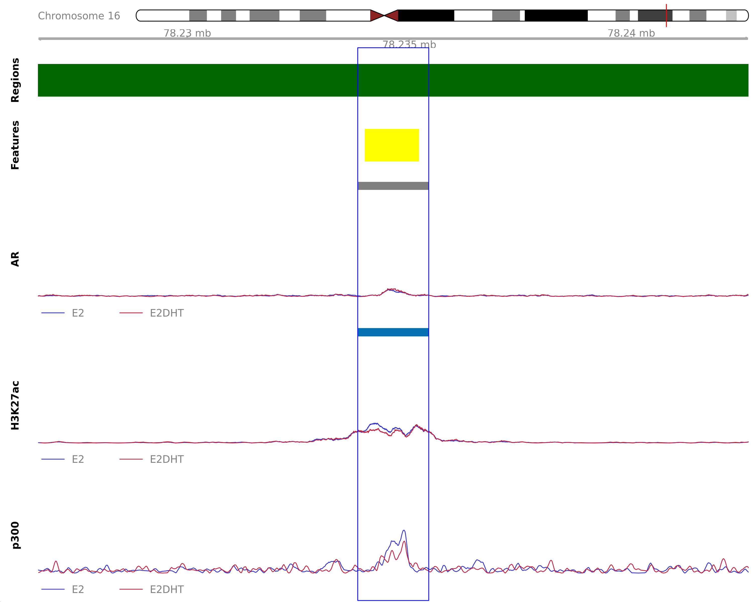
) AR Up - H3K27ac Up
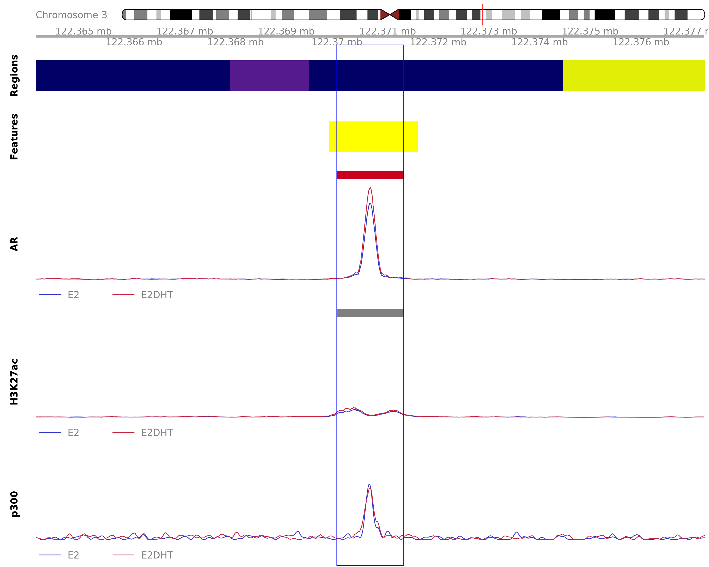
Highlighted region corresponds to the highest signal within the group AR Up - H3K27ac Up. The most likely target genes are DTX3L, HSPBAP1, PARP9 and PARP14
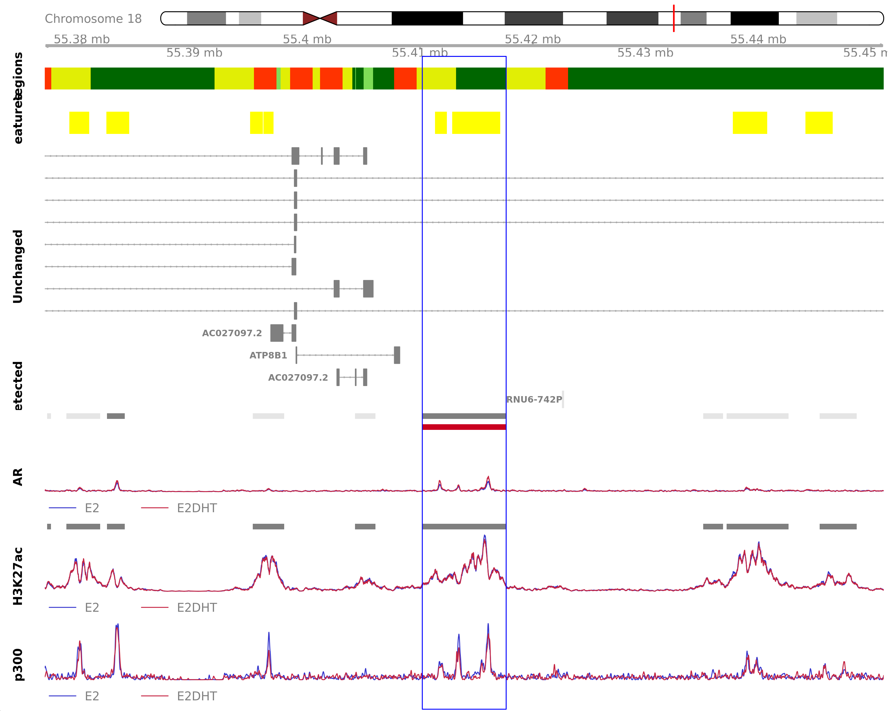
AR Up - H3K27ac Down
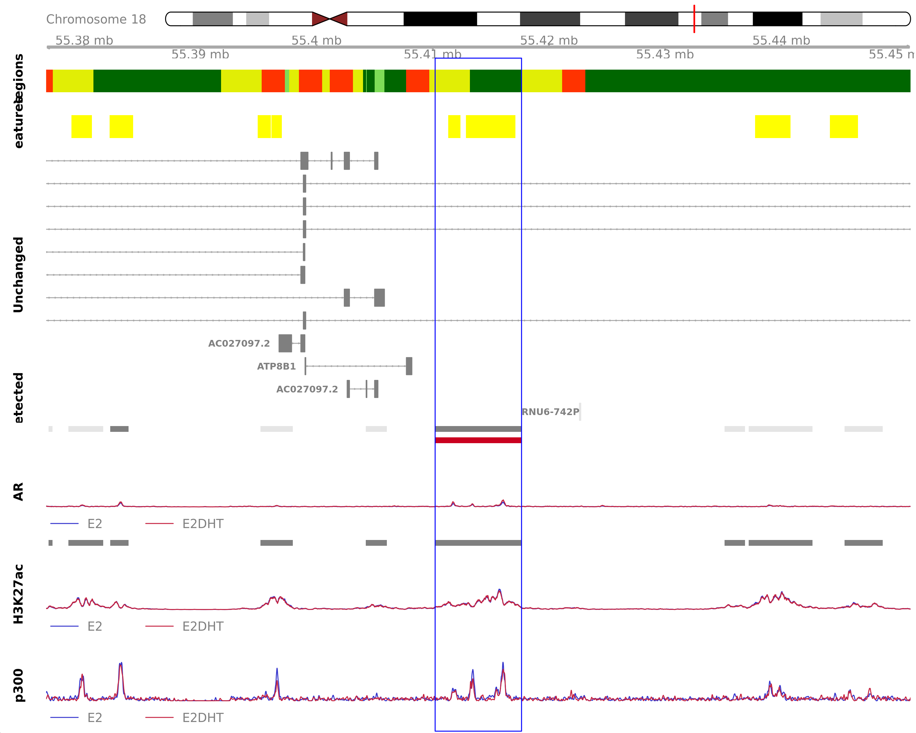
Highlighted region corresponds to the highest signal within the group AR Up - H3K27ac Down. The most likely target genes are AC027097.1, AC027097.2 and ATP8B1
AR Up - H3K27ac Unchanged
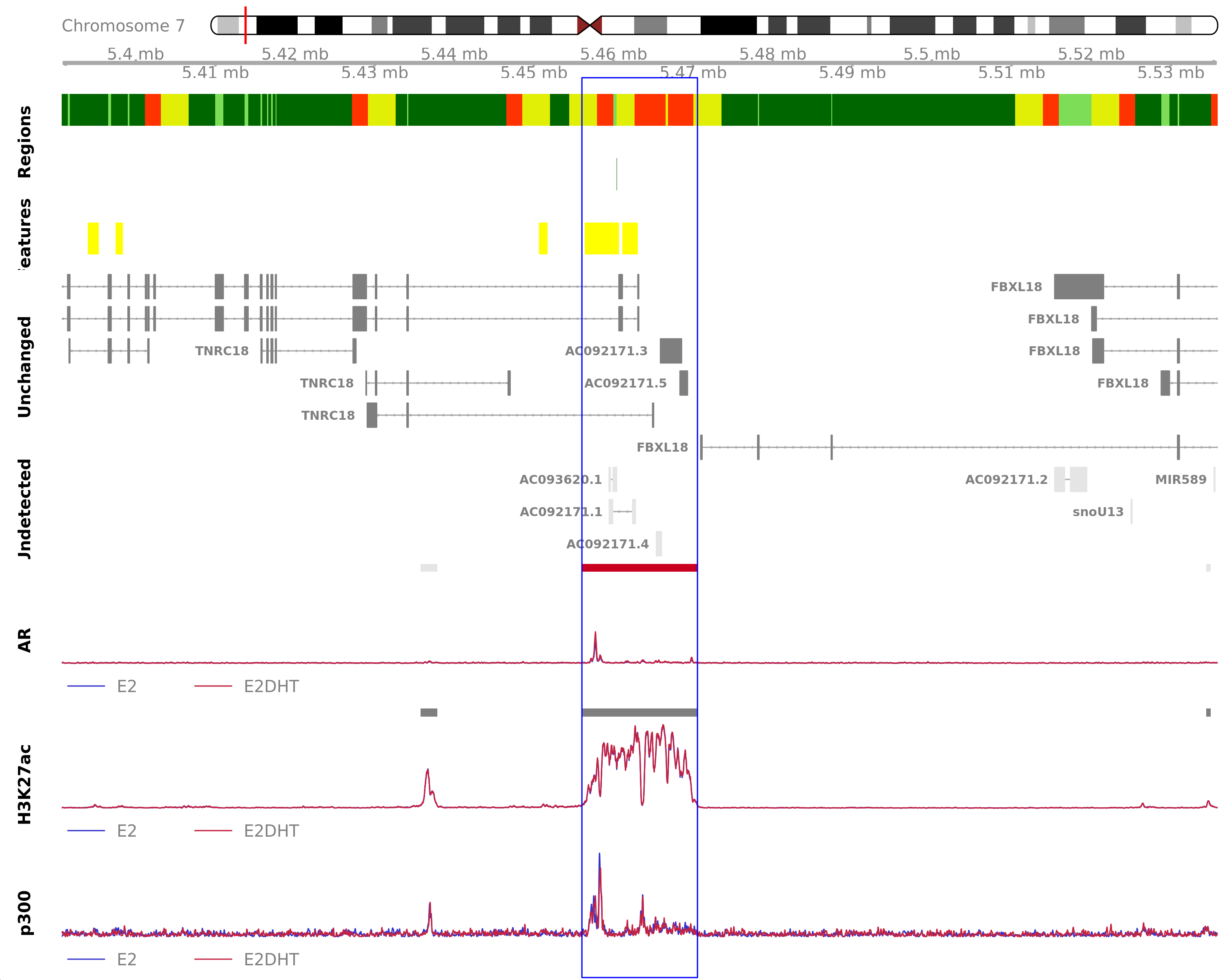
Highlighted region corresponds to the highest signal within the group AR Up - H3K27ac Unchanged. The most likely target genes are AC092171.3, AC092171.5, FBXL18 and TNRC18
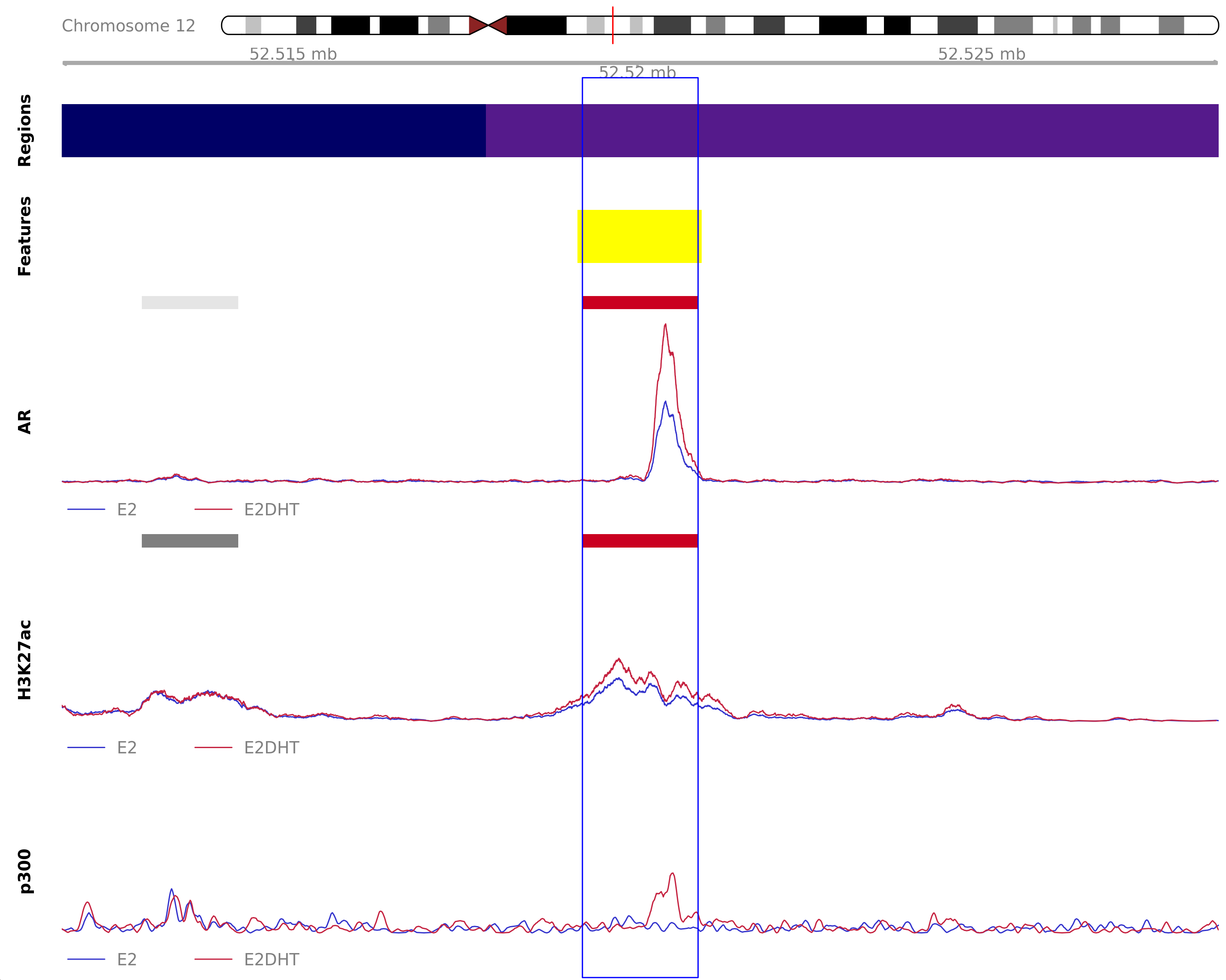
AR Unchanged - H3K27ac Down

Highlighted region corresponds to the highest signal within the group AR Unchanged - H3K27ac Down. The most likely target gene is WWOX
Windows With The Largest Change
For the initial set of visualisations, the sets of windows with the strongest signal were selected from within each group. Groups were restricted to those where differential binding was seen in at least comparison.
grl_to_plot <- all_windows %>%
  filter(
    !str_detect(status, "Un.+Un"),
    vapply(detected, length, integer(1)) > 0
  ) %>%
  as_tibble() %>%
  rename_all(
    str_replace_all, pattern = "\\.Vs\\.\\.", replacement = " Vs. "
  ) %>%
  rename_all(
    str_replace_all, pattern = "\\.\\.", replacement = ": "
  ) %>%
  nest(
    logFC = ends_with("logFC")
  ) %>%
  mutate(
    max_logFC = vapply(logFC, function(x) max(abs(unlist(x))), numeric(1))
  ) %>%
  group_by(status) %>%
  filter(max_logFC == max(max_logFC)) %>%
  dplyr::select(
    range, status, ends_with("logFC")
  ) %>%
  droplevels() %>%
  split(.$status) %>%
  lapply(pull, "range") %>%
  lapply(GRanges, seqinfo = sq) %>%
  GRangesList()
## Coverage y-limits
gr <- unlist(grl_to_plot)
y_lim <- lapply(
bwfl,
function(x) {
cov <- lapply(x, import.bw, which = gr)
unlist(lapply(cov, function(y) max(y$score))) %>%
c(0) %>%
range()
}
)
## External Coverage (Optional)
if (!is.null(config$external$coverage)) {
y_ranges <- grl_to_plot %>%
unlist() %>%
granges() %>%
resize(w = 10 * width(.), fix = 'center')
y_lim <- c(
y_lim[comps],
bwfl[names(config$external$coverage)] %>%
lapply(
function(x) {
GRangesList(lapply(x, import.bw, which = y_ranges)) %>%
unlist() %>%
filter(score == max(score)) %>%
mcols() %>%
.[["score"]] %>%
c(0) %>%
range()
}
)
)
}htmltools::tagList(
mclapply(
seq_along(grl_to_plot),
function(x) {
## Export the image
img_out <- file.path(
fig_path,
names(grl_to_plot)[[x]] %>%
str_remove_all("(:|Vs. |- )") %>%
str_replace_all(" ", "_") %>%
paste0("_logFC.", fig_type)
)
fig_fun(
filename = img_out, width = 10, height = 8
)
ct <- FALSE
if (length(subsetByOverlaps(gtf_transcript, grl_to_plot[[x]])) > 10)
ct <- "meta"
plotHFGC(
grl_to_plot[[x]],
features = feat_gr, featcol = feature_colours,
featsize = 1 + has_features,
genes = hfgc_genes, genecol = gene_col,
coverage = bwfl, linecol = line_col,
annotation = annot, annotcol = annot_col,
cytobands = bands_df,
rotation.title = 90,
zoom = 10,
ylim = y_lim,
collapseTranscripts = ct,
col.title = "black", background.title = "white", showAxis = FALSE
)
dev.off()
## Create html tags
fig_link <- str_extract(img_out, "assets.+")
gn <- unlist(subsetByOverlaps(all_windows, grl_to_plot[[x]])$detected)
cp <- htmltools::tags$em(
glue(
"
Highlighted region corresponds to the largest change within the group
{names(grl_to_plot)[[x]]}. The most likely target
{ifelse(length(gn) == 1, 'gene is ', 'genes are ')}
{collapseGenes(gn, format = '')}
"
)
)
htmltools::div(
htmltools::div(
id = names(grl_to_plot)[[x]] %>%
str_remove_all("(:|Vs. |- )") %>%
str_replace_all(" ", "-") %>%
str_to_lower() %>%
paste0("-logfc"),
class = "section level3",
htmltools::h3(names(grl_to_plot)[[x]]),
htmltools::div(
class = "figure", style = "text-align: center",
htmltools::img(src = fig_link, width = 960),
htmltools::p(
class = "caption", htmltools::tags$em(cp)
)
)
)
)
},
mc.cores = threads
)
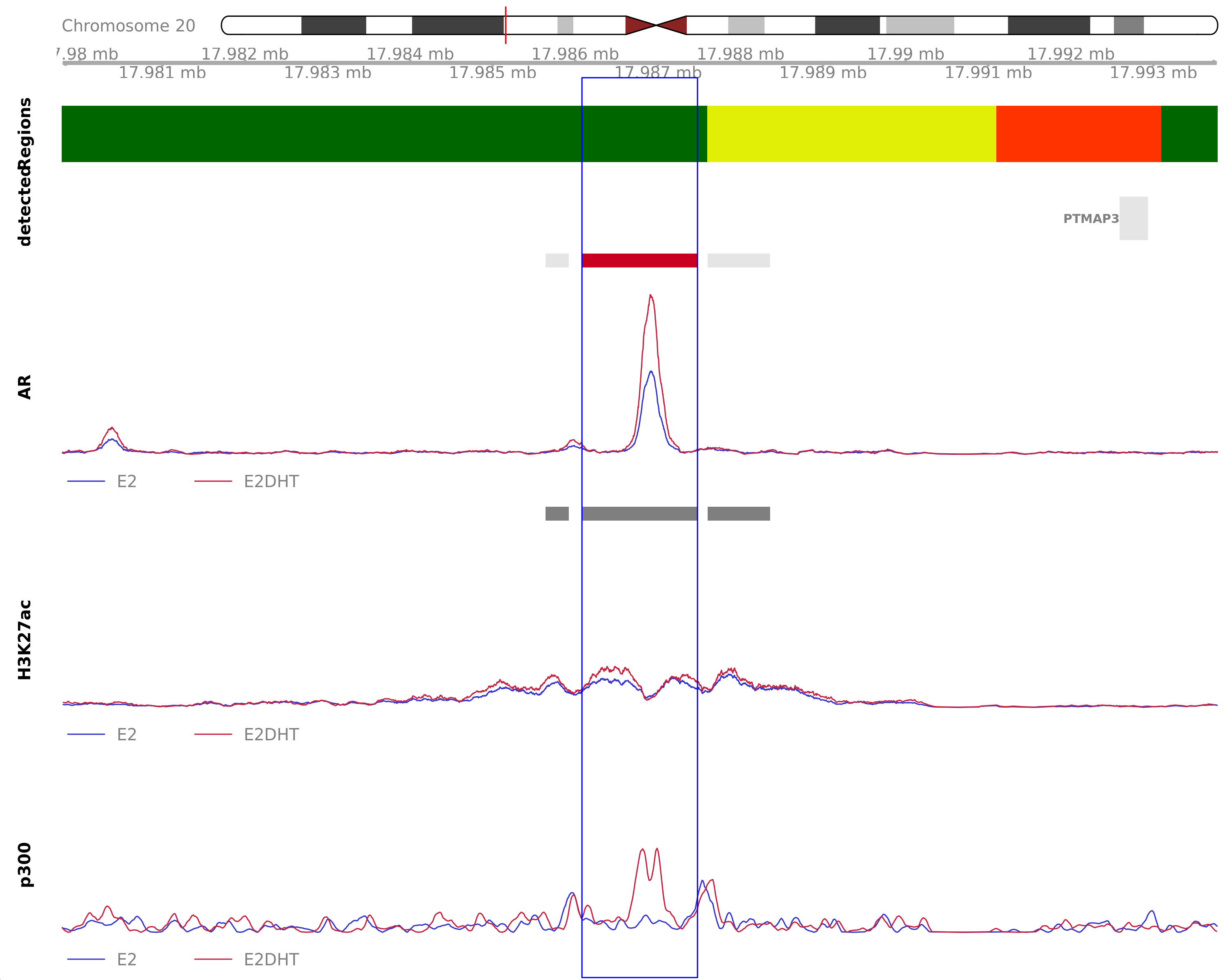
) AR Up - H3K27ac Up
Highlighted region corresponds to the largest change within the group AR Up - H3K27ac Up. The most likely target genes are ATG101, KRT80 and NR4A1
AR Up - H3K27ac Down
Highlighted region corresponds to the largest change within the group AR Up - H3K27ac Down. The most likely target genes are AC027097.1, AC027097.2 and ATP8B1
AR Up - H3K27ac Unchanged
Highlighted region corresponds to the largest change within the group AR Up - H3K27ac Unchanged. The most likely target genes are OVOL2
AR Unchanged - H3K27ac Down
Highlighted region corresponds to the largest change within the group AR Unchanged - H3K27ac Down. The most likely target gene is WWOX
Enrichment Analysis
min_gs_size <- extra_params$enrichment$min_size
if (is.null(min_gs_size) | is.na(min_gs_size)) min_gs_size <- 0
max_gs_size <- extra_params$enrichment$max_size
if (is.null(max_gs_size) | is.na(max_gs_size)) max_gs_size <- Inf
min_sig <- extra_params$enrichment$min_sig
if (is.null(min_sig) | is.na(min_sig)) min_sig <- 1

all_ids <- gtf_gene %>%
  mutate(w = width) %>%
  as_tibble() %>%
  dplyr::select(gene_id, w) %>%
  arrange(desc(w)) %>%
  distinct(gene_id, w) %>%
  arrange(gene_id) %>%
  left_join(
    all_windows$gene_id %>%
      unlist() %>%
      table() %>%
      enframe(name = "gene_id", value = "n_windows"),
    by = "gene_id"
  ) %>%
  dplyr::filter(gene_id %in% gtf_gene$gene_id) %>%
  mutate(
    n_windows = as.integer(ifelse(is.na(n_windows), 0, n_windows))
  )
msigdb <- msigdbr(species = extra_params$enrichment$species) %>%
  dplyr::filter(
    gs_cat %in% unlist(extra_params$enrichment$msigdb$gs_cat) |
      gs_subcat %in% unlist(extra_params$enrichment$msigdb$gs_subcat),
    str_detect(ensembl_gene, "^E")
  ) %>%
  dplyr::rename(gene_id = ensembl_gene, gene_name = gene_symbol) %>% # For easier integration
  dplyr::select(-starts_with("human"), -contains("entrez")) %>%
  dplyr::filter(gene_id %in% all_ids$gene_id) %>%
  group_by(gs_name) %>%
  mutate(n = dplyr::n()) %>%
  ungroup() %>%
  dplyr::filter(n >= min_gs_size, n <= max_gs_size)
gs_by_gsid <- msigdb %>%
  split(.$gs_name) %>%
  mclapply(pull, "gene_id", mc.cores = threads) %>%
  mclapply(unique, mc.cores = threads)
gs_by_geneid <- msigdb %>%
  split(.$gene_id) %>%
  mclapply(pull, "gs_name", mc.cores = threads) %>%
  mclapply(unique, mc.cores = threads)
gs_url <- msigdb %>%
  distinct(gs_name, gs_url) %>%
  mutate(
    gs_url = ifelse(
      gs_url == "", "
      http://www.gsea-msigdb.org/gsea/msigdb/collections.jsp",
      gs_url
    )
  ) %>%
  with(setNames(gs_url, gs_name))

min_network_size <- extra_params$networks$min_size
if (is.null(min_network_size) | is.na(min_network_size))
  min_network_size <- 2

max_network_size <- extra_params$networks$max_size
if (is.null(max_network_size) | is.na(max_network_size))
  max_network_size <- Inf

max_network_dist <- extra_params$networks$max_distance
if (is.null(max_network_dist) | is.na(max_network_dist))
  max_network_dist <- 1

net_layout <- extra_params$networks$layout
enrich_alpha <- extra_params$enrichment$alpha
adj_method <- match.arg(extra_params$enrichment$adj, p.adjust.methods)
adj_desc <- case_when(
  p.adjust.methods %in% c("fdr", "BH") ~ "the Benjamini-Hochberg FDR",
  p.adjust.methods %in% c("BY") ~ "the Benjamini-Yekutieli FDR",
  p.adjust.methods %in% c("bonferroni") ~ "the Bonferroni",
  p.adjust.methods %in% c("holm") ~ "Holm's",
  p.adjust.methods %in% c("hommel") ~ "Hommel's",
  p.adjust.methods %in% c("hochberg") ~ "Hochberg's",
  p.adjust.methods %in% c("none") ~ "no"
) %>%
  setNames(p.adjust.methods)
comp_ids <- comps %>%
  lapply(
    function(x) {
      subset(all_windows, !str_detect(status, paste(x, "Undetected")))$gene_id
    }
  ) %>%
  lapply(unlist) %>%
  lapply(unique) %>%
  lapply(intersect, gtf_gene$gene_id) %>%
  setNames(comps)
mapped_ids <- comp_ids %>%
  unlist() %>%
  unique()
gene_lengths <- structure(width(gtf_gene), names = gtf_gene$gene_id)[mapped_ids]
group_ids <- all_windows %>%
  split(f = .$status) %>%
  mclapply(
    function(x) unique(unlist(x$gene_id)),
    mc.cores = threads
  )
Comparison of Genes Mapped To Targets
The first level of enrichment testing performed was to simply check the genes mapped to a binding site in either comparison, with no consideration being paid to the dynamics of binding in either comparison. This will capture and describe the overall biological activity being jointly regulated.
The genes in each section and intersection in the following Venn
Diagram will then be analysed against the complete set of 12,436 genes
mapped to either AR or H3K27ac. Firstly, all 12,436 genes mapped to a
binding site were tested for enrichment in comparison to the set of
12,990 detected genes. For this analysis, gene width was used as a
potential source of sampling bias and Wallenius’ Non-Central
Hypergeometric was used as implemented in goseq (Young et al. 2010).
The sets of genes mapped to each section of the Venn Diagram were then tested for enrichment in comparison to the larger set of 12,436 mapped genes. The standard hypergeometric distribution was used for these analyses.
If 4 or more gene-sets were considered to be enriched, a network plot was produced using the same methodology as for results from differential binding for individual comparisons.
plotOverlaps(
  comp_ids, set_col = comp_cols[comps], cex = 1.2, cat.cex = 1.2
)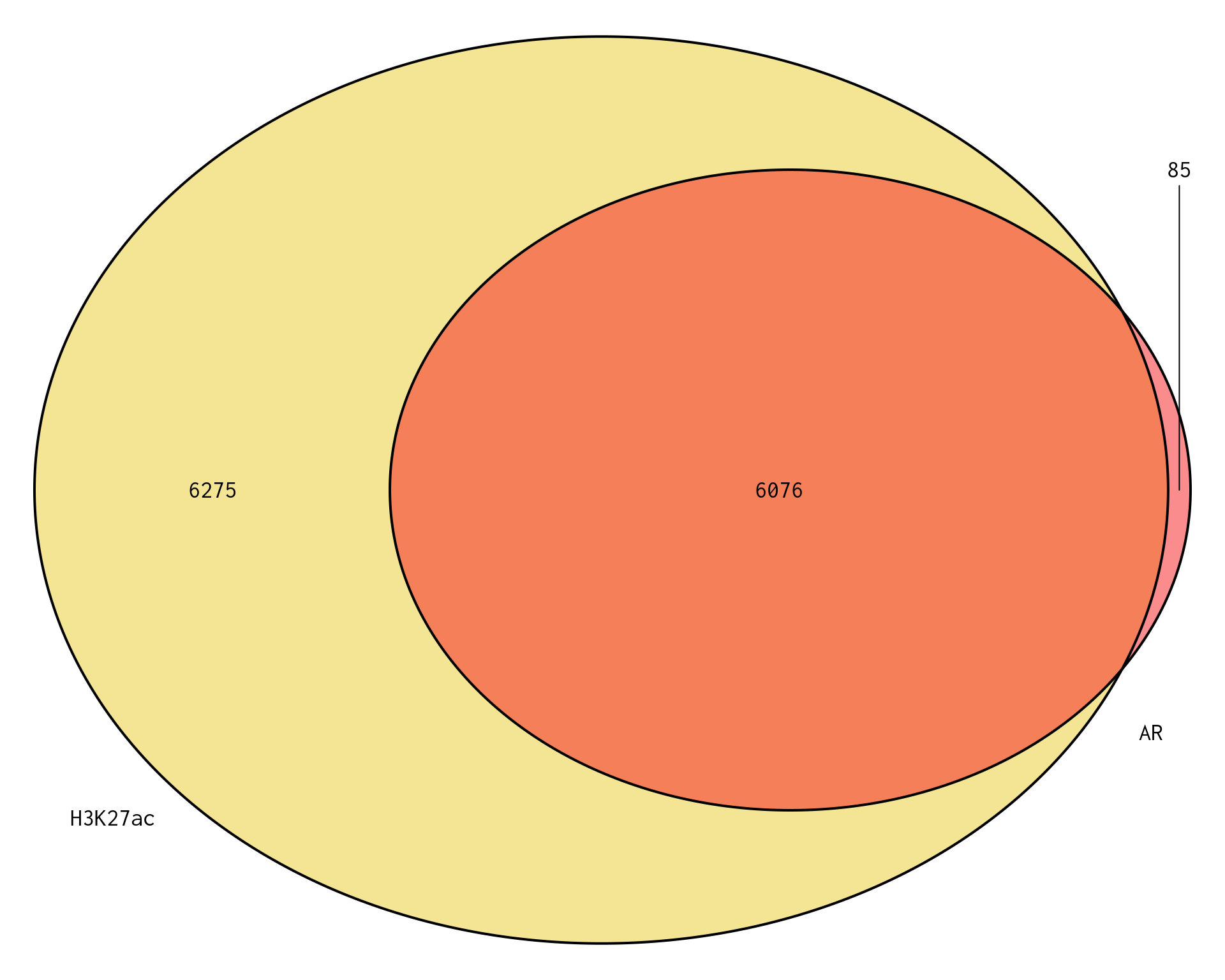
Venn Diagram showing genes mapped to a binding region associated with AR or H3K27ac. Of the 12,990 genes under consideration, a total of 12,436 genes were mapped to a binding region across both comparisons, leaving 554 genes unmapped to a binding region across either comparison.
Result Tables
Mapped Genes To Either AR or H3K27ac
pwf_mapped <- gtf_gene %>%
  mutate(w = width) %>%
  as_tibble() %>%
  arrange(gene_id, desc(w)) %>%
  distinct(gene_id, w) %>%
  mutate(mapped = gene_id %in% mapped_ids) %>%
  with(nullp(setNames(mapped, gene_id), bias.data = log10(w)))
goseq_mapped_res <- pwf_mapped %>%
goseq(gene2cat = gs_by_geneid) %>%
dplyr::filter(numDEInCat > 0) %>%
as_tibble() %>%
dplyr::select(
gs_name = category, pval = over_represented_pvalue, starts_with("num")
) %>%
mutate(
adj_p = p.adjust(pval, adj_method),
enriched = adj_p < enrich_alpha
) %>%
dplyr::filter(numDEInCat >= min_sig) %>%
left_join(
dplyr::filter(msigdb, gene_id %in% mapped_ids)[c("gs_name", "gene_name", "gs_url", "gs_description")],
by = "gs_name"
) %>%
chop(gene_name) %>%
mutate(
gene_name = vapply(gene_name, paste, character(1), collapse = "; ")
)
any_goseq_mapped <- sum(goseq_mapped_res$adj_p < enrich_alpha) > 0
tg_mapped <- make_tbl_graph(
goseq_mapped_res,
gs = gs_by_gsid %>%
lapply(intersect, rownames(subset(pwf_mapped, DEgenes))) %>%
.[vapply(., length, integer(1)) > 0]
)
plot_network_mapped <- length(tg_mapped) >= min_network_sizeNo pathway enrichment was detected amongst genes mapped in either comparison.
Genes Mapped to Both AR and H3K27ac
pwf_t1t2 <- nullp(
  vec_t1t2,
  bias.data = log10(setNames(all_ids$w, all_ids$gene_id)[mapped_ids]),
  plot.fit = TRUE
)
if (sum(pwf_t1t2$DEgenes) > 0) {
goseq_t1t2_res <- pwf_t1t2 %>%
goseq(gene2cat = gs_by_geneid, method = gs_method) %>%
dplyr::filter(numDEInCat > 0) %>%
as_tibble() %>%
dplyr::select(
gs_name = category, pval = over_represented_pvalue, starts_with("num")
) %>%
mutate(
adj_p = p.adjust(pval, adj_method),
enriched = adj_p < enrich_alpha
) %>%
dplyr::filter(numDEInCat >= min_sig) %>%
left_join(
dplyr::filter(msigdb, gene_id %in% mapped_ids)[c("gs_name", "gene_name", "gs_url", "gs_description")],
by = "gs_name"
) %>%
chop(gene_name) %>%
mutate(gene_name = vapply(gene_name, paste, character(1), collapse = "; "))
}
any_goseq_t1t2 <- sum(goseq_t1t2_res$adj_p < enrich_alpha) > 0
tg_t1t2 <- make_tbl_graph(
goseq_t1t2_res,
gs = gs_by_gsid %>%
lapply(intersect, rownames(subset(pwf_t1t2, DEgenes))) %>%
.[vapply(., length, integer(1)) > 0]
)
plot_network_t1t2 <- length(tg_t1t2) >= min_network_size
if (!any_goseq_t1t2) para <- glue(para, " No enrichment was found.")tbl <- goseq_t1t2_res %>%
dplyr::filter(enriched) %>%
dplyr::select(
gs_name, gs_description, pval, adj_p, starts_with("num"), gene_name
) %>%
reactable(
filterable = TRUE,
showPageSizeOptions = TRUE,
columns = list2(
gs_name = colDef(
name = "Gene Set",
cell = function(value) htmltools::tags$a(
href = gs_url[[value]],
target = "_blank",
str_replace_all(value, "_", " ")
),
html = TRUE,
maxWidth = 150
),
gs_description = colDef(
name = "Description",
cell = function(value) str_trunc(value, width = 150)
),
pval = colDef(
name = "P-Value",
cell = function(value) ifelse(
value < 0.001,
sprintf("%.2e", value),
sprintf("%.3f", value)
),
maxWidth = 80
),
adj_p = colDef(
name = "p<sub>adj</sub>", html = TRUE,
cell = function(value) ifelse(
value < 0.001,
sprintf("%.2e", value),
sprintf("%.3f", value)
),
maxWidth = 80
),
numDEInCat = colDef(
name = "Genes Mapped to Both",
cell = function(value) comma(value, 1),
maxWidth = 80
),
numInCat = colDef(
name = "Genes Mapped to Either",
cell = function(value) comma(value, 1),
maxWidth = 80
),
gene_name = colDef(
name = "Gene Names",
cell = function(value) with_tooltip(value, width = 150)
)
)
)
div(class = "table",
div(class = "table-header", div(class = "caption", para)),
tbl
)Genes Mapped to AR Only
goseq_t1only_res <- tibble(
  gs_name = character(), mapped = numeric(), enriched = logical(),
  adj_p = numeric()
)
vec_t1only <- structure(
  mapped_ids %in% setdiff(comp_ids[[1]], comp_ids[[2]]),
  names = mapped_ids
)
gs_method <- "Hypergeometric"
any_goseq_t1only <- plot_network_t1only <- FALSE
para <- glue(
  "
  All {comma(length(setdiff(comp_ids[[1]], comp_ids[[2]])))} genes with a
  mapped binding window to only {comps[[1]]} were compared to
  the {comma(length(mapped_ids))} genes mapped to either
  {glue_collapse(comps, last = ' or ')}, in order to ascertain whether any gene-sets
  were likely to be targeted exclusively. No sampling bias offset was
  incorporated, instead using a simple Hypergeometric model for enrichment testing.
  "
)
pwf_t1only <- nullp(
vec_t1only,
bias.data = log10(setNames(all_ids$w, all_ids$gene_id)[mapped_ids]),
plot.fit = TRUE
) if (sum(pwf_t1only$DEgenes) > 0) {
goseq_t1only_res <- pwf_t1only %>%
goseq(gene2cat = gs_by_geneid, method = gs_method) %>%
dplyr::filter(numDEInCat > 0) %>%
as_tibble() %>%
dplyr::select(
gs_name = category, pval = over_represented_pvalue, starts_with("num")
) %>%
mutate(
adj_p = p.adjust(pval, adj_method),
enriched = adj_p < enrich_alpha
) %>%
dplyr::filter(numDEInCat >= min_sig) %>%
left_join(
dplyr::filter(msigdb, gene_id %in% mapped_ids)[c("gs_name", "gene_name", "gs_url", "gs_description")],
by = "gs_name"
) %>%
chop(gene_name) %>%
mutate(gene_name = vapply(gene_name, paste, character(1), collapse = "; "))
}
any_goseq_t1only <- sum(goseq_t1only_res$adj_p < enrich_alpha) > 0
tg_t1only <- make_tbl_graph(
goseq_t1only_res,
gs = gs_by_gsid %>%
lapply(intersect, rownames(subset(pwf_t1only, DEgenes))) %>%
.[vapply(., length, integer(1)) > 0]
)
plot_network_t1only <- length(tg_t1only) >= min_network_size
if (!any_goseq_t1only) para <- glue(para, " No enrichment was found.")All 85 genes with a mapped binding window to only AR were compared to the 12,436 genes mapped to either AR or H3K27ac, in order to ascertain whether any gene-sets were likely to be targeted exclusively. No sampling bias offset was incorporated, instead using a simple Hypergeometric model for enrichment testing. No enrichment was found.
Genes Mapped to H3K27ac Only
goseq_t2only_res <- tibble(
  gs_name = character(), mapped = numeric(), enriched = logical(),
  adj_p = numeric()
)
vec_t2only <- structure(
  mapped_ids %in% setdiff(comp_ids[[2]], comp_ids[[1]]),
  names = mapped_ids
)
gs_method <- "Hypergeometric"
para <- glue(
  "
  All {comma(length(setdiff(comp_ids[[2]], comp_ids[[1]])))} genes with a
  mapped binding window to only {comps[[2]]} were compared to
  the {comma(length(mapped_ids))} genes mapped to either
  {glue_collapse(comps, last = ' or ')}, in order to ascertain whether any gene-sets
  were likely to be targeted exclusively. No sampling bias offset was
  incorporated, instead using a simple Hypergeometric model for enrichment testing.
  "
)
any_goseq_t2only <- plot_network_t2only <- FALSE
pwf_t2only <- nullp(
vec_t2only,
bias.data = log10(setNames(all_ids$w, all_ids$gene_id)[mapped_ids]),
plot.fit = TRUE
) if (sum(pwf_t2only$DEgenes) > 0) {
goseq_t2only_res <- pwf_t2only %>%
goseq(gene2cat = gs_by_geneid, method = gs_method) %>%
dplyr::filter(numDEInCat > 0) %>%
as_tibble() %>%
dplyr::select(
gs_name = category, pval = over_represented_pvalue, starts_with("num")
) %>%
mutate(
adj_p = p.adjust(pval, adj_method),
enriched = adj_p < enrich_alpha
) %>%
dplyr::filter(numDEInCat >= min_sig) %>%
left_join(
dplyr::filter(msigdb, gene_id %in% mapped_ids)[c("gs_name", "gene_name", "gs_url", "gs_description")],
by = "gs_name"
) %>%
chop(gene_name) %>%
mutate(gene_name = vapply(gene_name, paste, character(1), collapse = "; "))
}
any_goseq_t2only <- sum(goseq_t2only_res$adj_p < enrich_alpha) > 0
tg_t2only <- make_tbl_graph(
goseq_t2only_res,
gs = gs_by_gsid %>%
lapply(intersect, rownames(subset(pwf_t2only, DEgenes))) %>%
.[vapply(., length, integer(1)) > 0]
)
plot_network_t2only <- length(tg_t2only) >= min_network_size
if (!any_goseq_t2only) para <- glue(para, " No enrichment was found.")tbl <- goseq_t2only_res %>%
dplyr::filter(enriched) %>%
dplyr::select(
gs_name, gs_description, pval, adj_p, starts_with("num"), gene_name
) %>%
reactable(
filterable = TRUE,
showPageSizeOptions = TRUE,
columns = list2(
gs_name = colDef(
name = "Gene Set",
cell = function(value) htmltools::tags$a(
href = gs_url[[value]],
target = "_blank",
str_replace_all(value, "_", " ")
),
html = TRUE,
maxWidth = 150
),
gs_description = colDef(
name = "Description",
cell = function(value) str_trunc(value, width = 150)
),
pval = colDef(
name = "P-Value",
cell = function(value) ifelse(
value < 0.001,
sprintf("%.2e", value),
sprintf("%.3f", value)
),
maxWidth = 80
),
adj_p = colDef(
name = "p<sub>adj</sub>", html = TRUE,
cell = function(value) ifelse(
value < 0.001,
sprintf("%.2e", value),
sprintf("%.3f", value)
),
maxWidth = 80
),
numDEInCat = colDef(
name = glue("Genes Mapped to {comps[[2]]} Only"),
cell = function(value) comma(value, 1),
maxWidth = 80
),
numInCat = colDef(
name = "Genes Mapped to Both",
cell = function(value) comma(value, 1),
maxWidth = 80
),
gene_name = colDef(
name = "Gene Names",
cell = function(value) with_tooltip(value, width = 150)
)
)
)
div(class = "table",
div(class = "table-header", div(class = "caption", para)),
tbl
)Network Plots
Genes Mapped to Both AR and H3K27ac
tg_t1t2 %>%
  ggraph(layout = net_layout, weights = oc^2) +
  geom_edge_link(aes(width = oc^2, alpha = oc^2)) +
  geom_node_point(
    aes(fill = -log10(pval), size = numDEInCat),
    shape = 21
  ) +
  geom_node_text(
    aes(label = label),
    colour = "black", size = 3,
    data = . %>%
      mutate(
        label = str_replace_all(label, "_", " ") %>% str_trunc(60) %>% str_wrap(width = 18)
      ),
    repel = TRUE, max.overlaps = max(10, round(length(tg_t1t2) / 4, 0)),
    bg.color = "white", bg.r = 0.1,
  ) +
  scale_x_continuous(expand = expansion(c(0.1, 0.1))) +
  scale_y_continuous(expand = expansion(c(0.1, 0.1))) +
  scale_fill_viridis_c(option = "inferno", begin = 0.25) +
  scale_size_continuous(range = c(1, 10)) +
  scale_edge_width(range = c(1, 6), limits = c(0, 1)) +
  scale_edge_alpha(range = c(0.1, 0.4), limits = c(0, 1)) +
  guides(edge_alpha = "none") +
  labs(size = "Mapped Genes", edge_width = expr(paste(OC^2))) +
theme_void() 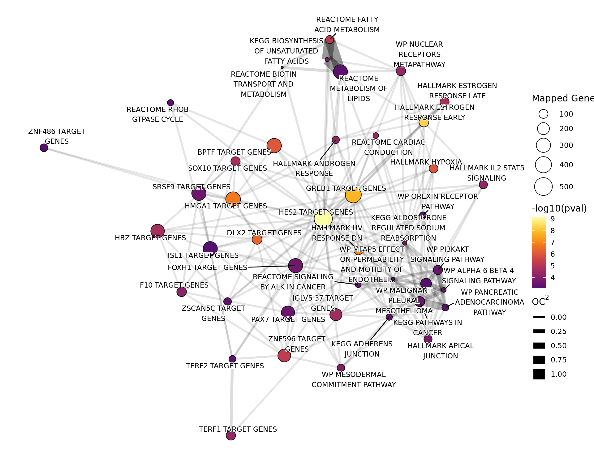
Network plot showing gene-sets enriched amongst the overall set of sites with a binding site for both AR and H3K27ac.
Genes Mapped to H3K27ac Only
tg_t2only %>%
  ggraph(layout = net_layout, weights = oc^2) +
  geom_edge_link(aes(width = oc^2, alpha = oc^2)) +
  geom_node_point(
    aes(fill = -log10(pval), size = numDEInCat),
    shape = 21
  ) +
  geom_node_text(
    aes(label = label),
    colour = "black", size = 3,
    data = . %>%
      mutate(
        label = str_replace_all(label, "_", " ") %>% str_trunc(60) %>% str_wrap(width = 18)
      ),
    repel = TRUE, max.overlaps = max(10, round(length(tg_t2only) / 4, 0)),
    bg.color = "white", bg.r = 0.1,
  ) +
  scale_x_continuous(expand = expansion(c(0.1, 0.1))) +
  scale_y_continuous(expand = expansion(c(0.1, 0.1))) +
  scale_fill_viridis_c(option = "inferno", begin = 0.25) +
  scale_size_continuous(range = c(1, 10)) +
  scale_edge_width(range = c(1, 6), limits = c(0, 1)) +
  scale_edge_alpha(range = c(0.1, 0.4), limits = c(0, 1)) +
  guides(edge_alpha = "none") +
  labs(size = "Mapped Genes", edge_width = expr(paste(OC^2))) +
theme_void() 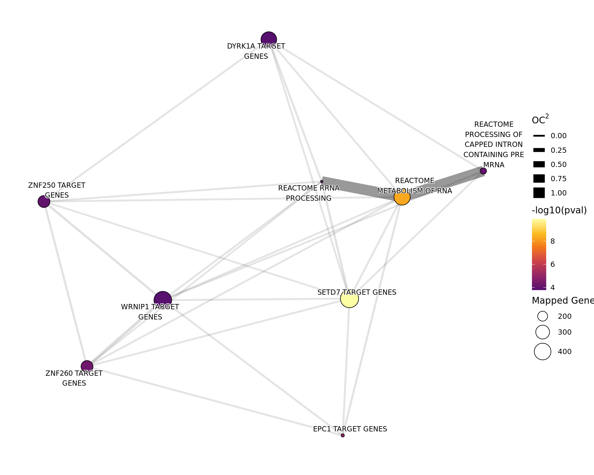
Network plot showing all gene-sets enriched amongst the overall set of sites with a binding site for H3K27ac only.
Comparison of Differentially Bound Windows
n_peaks <- structure(all_ids$n_windows, names = all_ids$gene_id)[mapped_ids]
goseq_group_res <- group_ids %>%
  .[str_detect(names(.), "Up|Down")] %>%
  mclapply(
    function(x) {
      vec <- structure(mapped_ids %in% x, names = mapped_ids)
      pwf <- nullp(vec, bias.data = n_peaks, plot.fit = FALSE)
      res <- tibble(adj_p = numeric())
      gs_method <- "Hypergeometric"
      if (sum(pwf$DEgenes) > 0) {
        res <- goseq(pwf, gene2cat = gs_by_geneid, method = gs_method) %>%
          as_tibble() %>%
          dplyr::filter(numDEInCat > 0) %>%
          mutate(adj_p = p.adjust(over_represented_pvalue, adj_method)) %>%
          dplyr::filter(numDEInCat >= min_sig) %>%
          dplyr::select(
            gs_name = category, pval = over_represented_pvalue, adj_p,
            ends_with("InCat")
          ) %>%
          left_join(
            dplyr::filter(msigdb, gene_id %in% x)[c("gs_name", "gene_name", "gs_url", "gs_description")],
            by = "gs_name"
          ) %>%
          chop(gene_name) %>%
          mutate(
            gene_name = vapply(gene_name, paste, character(1), collapse = "; ")
          )
      }
      res
    },
    mc.cores = threads
  ) %>%
  ## This step at the end basically removes any groups with no results
  lapply(list) %>%
  as_tibble() %>%
  pivot_longer(everything(), names_to = "group") %>%
  unnest(everything()) %>%
  split(.$group)
goseq_group_sig <- goseq_group_res %>%
  lapply(dplyr::filter, adj_p < enrich_alpha) %>%
  .[vapply(., nrow, integer(1)) > 0]
tg_group_res <- names(goseq_group_sig) %>%
  lapply(
    function(x) {
      make_tbl_graph(
        goseq_group_sig[[x]],
        gs_by_gsid[goseq_group_sig[[x]]$gs_name] %>%
          lapply(intersect, group_ids[[x]])
      )
    }
  ) %>%
  setNames(names(goseq_group_sig)) %>%
  .[vapply(., length, integer(1)) >= min_network_size]
The same MSigDB gene sets were used for associating any pathways with the combined changes in both AR and H3K27ac. The ‘universe’ of genes was defined as all 12,436 gene ids with a binding window mapped from either target. No sampling bias was included, with test results using a simple Hypergeometric Distribution.
Results
htmltools::tagList(
  names(goseq_group_sig) %>%
    mclapply(
      function(x) {
        cp <- glue(
          "
          All {comma(length(group_ids[[x]]), 1)} genes mapped to binding windows
           with the pattern {x} were compared to the complete set of
          {comma(length(mapped_ids), 1)} genes mapped to at least one binding
          window. {nrow(goseq_group_sig[[x]])} gene-sets were considered as
          enriched using a threshold of {enrich_alpha} for adjusted-p-values.
          "
        )
        htmltools::div(
          htmltools::div(
            id = x %>%
              str_to_lower %>%
              str_replace_all(" ", "-") %>%
              str_replace_all("-+", "-"),
            class = "section level4",
            htmltools::h4(class = "tabset", x),
            htmltools::tags$em(cp),
            goseq_group_sig[[x]] %>%
              separate(group, into = comps, sep = " - ") %>%
              dplyr::select(
                all_of(comps), gs_name, gs_description, pval, adj_p, everything()
              ) %>%
              reactable(
                filterable = TRUE,
                showPageSizeOptions = TRUE,
                columns = list2(
                  "{comps[[1]]}" := colDef(
                    cell = function(value) {
                      value <- str_extract(value, "Up|Down|Unchanged|Undetected")
                      if (str_detect(value, "Up")) value <- paste(value, "\u21E7")
                      if (str_detect(value, "Down")) value <- paste(value, "\u21E9")
                      paste(targets[[1]], value)
                    },
                    style = function(value) {
                      colour <- case_when(
                        str_detect(value, "Up") ~ colours$direction[["up"]],
                        str_detect(value, "Down") ~ colours$direction[["down"]],
                        str_detect(value, "Unchanged") ~ colours$direction[["unchanged"]],
                        str_detect(value, "Undetected") ~ colours$direction[["undetected"]]
                      )
                      list(color = colour)
                    },
                    maxWidth = 120
                  ),
                  "{comps[[2]]}" := colDef(
                    cell = function(value) {
                      value <- str_extract(value, "Up|Down|Unchanged|Undetected")
                      if (str_detect(value, "Up")) value <- paste(value, "\u21E7")
                      if (str_detect(value, "Down")) value <- paste(value, "\u21E9")
                      paste(targets[[2]], value)
                    },
                    style = function(value) {
                      colour <- case_when(
                        str_detect(value, "Up") ~ colours$direction[["up"]],
                        str_detect(value, "Down") ~ colours$direction[["down"]],
                        str_detect(value, "Unchanged") ~ colours$direction[["unchanged"]],
                        str_detect(value, "Undetected") ~ colours$direction[["undetected"]]
                      )
                      list(color = colour)
                    },
                    maxWidth = 120
                  ),
                  gs_name = colDef(
                    name = "Gene Set",
                    cell = function(value) {
                      htmltools::tags$a(
                        href = gs_url[[value]], target = "_blank",
                        str_replace_all(value, "_", " ")
                      )
                    },
                    html = TRUE,
                    maxWidth = 150
                  ),
                  gs_description = colDef(
                    name = "Description",
                    cell = function(value) str_trunc(value, width = 150)
                  ),
                  gs_url = colDef(show = FALSE),
                  pval = colDef(
                    name = "P-Value",
                    cell = function(value) ifelse(
                      value < 0.001,
                      sprintf("%.2e", value),
                      sprintf("%.3f", value)
                    ),
                    maxWidth = 80
                  ),
                  adj_p = colDef(
                    name = "p<sub>adj</sub>", html = TRUE,
                    cell = function(value) ifelse(
                      value < 0.001,
                      sprintf("%.2e", value),
                      sprintf("%.3f", value)
                    ),
                    maxWidth = 80
                  ),
                  numDEInCat = colDef(
                    name = "Mapped Genes",
                    cell = function(value) comma(value, 1),
                    maxWidth = 80
                  ),
                  numInCat = colDef(
                    name = "Genes in Gene-Set",
                    cell = function(value) comma(value, 1),
                    maxWidth = 80
                  ),
                  gene_name = colDef(
                    name = "Gene Names",
                    cell = function(value) with_tooltip(value, width = 150)
                  )
                )
              )
          )
        )
      },
      mc.cores = threads
    )
)
AR Up - H3K27ac Unchanged
All 3,181 genes mapped to binding windows with the pattern AR Up - H3K27ac Unchanged were compared to the complete set of 12,436 genes mapped to at least one binding window. 5 gene-sets were considered as enriched using a threshold of 0.05 for adjusted-p-values.AR Up - H3K27ac Undetected
All 2,718 genes mapped to binding windows with the pattern AR Up - H3K27ac Undetected were compared to the complete set of 12,436 genes mapped to at least one binding window. 27 gene-sets were considered as enriched using a threshold of 0.05 for adjusted-p-values.AR Up - H3K27ac Up
All 477 genes mapped to binding windows with the pattern AR Up - H3K27ac Up were compared to the complete set of 12,436 genes mapped to at least one binding window. 3 gene-sets were considered as enriched using a threshold of 0.05 for adjusted-p-values.All Groups
goseq_group_sig %>%
  bind_rows() %>%
  arrange(pval) %>%
  left_join(n_mapped, by = c("group" = "status")) %>%
  mutate(
    gs_name = fct_inorder(gs_name) %>%
      fct_relabel(str_replace_all, "_", " ") %>%
      fct_relabel(str_trunc, width = 60),
    prop = numDEInCat / mapped,
    group = factor(group, levels = n_mapped$status)
  ) %>%
  droplevels() %>%
  ggplot(aes(group, fct_rev(gs_name))) +
  geom_point(aes(size = prop, fill = -log10(pval)), shape = 21) +
  geom_ysidecol(
    aes(x = numInCat), data = . %>% distinct(gs_name, numInCat),
  ) +
  geom_xsidecol(
    aes(y = mapped),
    data = n_mapped %>%
      dplyr::filter(status %in% names(goseq_group_sig)) %>%
      dplyr::rename(group = status),
    width = 0.5
  ) +
  scale_x_discrete(labels = label_wrap(10)) +
  scale_ysidex_continuous(expand = expansion(c(0, 0.15))) +
  scale_xsidey_continuous(
    expand = expansion(c(0, 0.15))
  ) +
  scale_fill_viridis_c(option = "inferno", begin = 0.2) +
  scale_size(range = c(0, 5), labels = percent) +
  labs(
    x = c(), y = c(), size = "% Mapped\nGenes", fill = expr(paste(-log[10], "p"))
  ) +
  theme(
    panel.grid = element_blank(),
    axis.text = element_text(size = 8),
    legend.position = "right",
    ggside.panel.scale.x = 0.2,
    ggside.panel.scale.y = 0.3,
    ggside.axis.text.x.bottom = element_text(angle = 270, hjust = 0, vjust = 0.5)
) 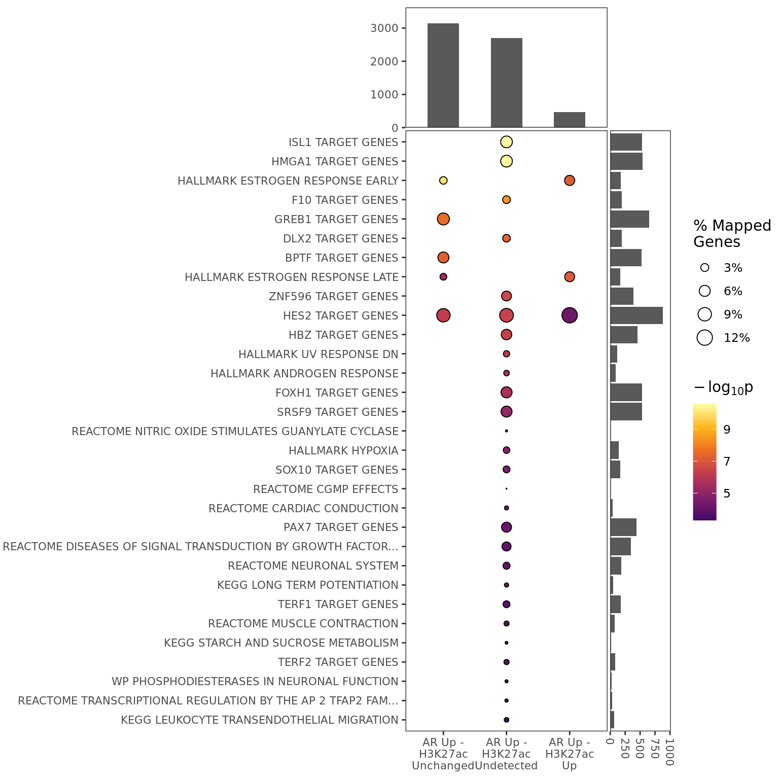
Combined enrichment across all groups, showing only significant results for enrichment. The top panel shows how many genes were mapped to sites for each group, whilst the right panel shows gene set size. Point sizes indicate the proportion of mapped genes which are from each pathway.
Network Plots
htmltools::tagList(
  names(tg_group_res) %>%
    mclapply(
      function(x) {
        ## Export the image
        img_out <- file.path(
          fig_path,
          x %>%
            str_replace_all(" ", "_") %>%
            str_replace_all("_-_", "-") %>%
            paste0("_network.", fig_type)
        )
        fig_fun(
          filename = img_out,
          width = knitr::opts_current$get("fig.width"),
          height = knitr::opts_current$get("fig.height")
        )
        p <- tg_group_res[[x]] %>%
          ggraph(layout = net_layout, weights = oc^2) +
          geom_edge_link(aes(width = oc^2, alpha = oc^2)) +
          geom_node_point(
            aes(fill = -log10(pval), size = numDEInCat),
            shape = 21
          ) +
          geom_node_text(
            aes(label = label),
            colour = "black", size = 3,
            data = . %>%
              mutate(
                label = str_replace_all(label, "_", " ") %>% str_trunc(60) %>% str_wrap(width = 18)
              ),
            repel = TRUE,
            max.overlaps = max(10, round(length(tg_group_res[[x]]) / 4, 0)),
            bg.color = "white", bg.r = 0.1
          ) +
          scale_x_continuous(expand = expansion(c(0.1, 0.1))) +
          scale_y_continuous(expand = expansion(c(0.1, 0.1))) +
          scale_fill_viridis_c(option = "inferno", begin = 0.25) +
          scale_size_continuous(range = c(1, 10)) +
          scale_edge_width(range = c(1, 6), limits = c(0, 1)) +
          scale_edge_alpha(range = c(0.1, 0.4), limits = c(0, 1)) +
          guides(edge_alpha = "none") +
          labs(size = "Mapped Genes", edge_width = expr(paste(OC^2))) +
          theme_void()
        print(p)
        dev.off()
        ## Create html tags
        fig_link <- str_extract(img_out, "assets.+")
        cp <- htmltools::tags$em(
          glue(
            "
            Network plot showing enriched pathways mapped to genes
            associated with {x}.
            "
          )
        )
        htmltools::div(
          htmltools::div(
            id = img_out %>%
              basename() %>%
              str_remove_all(glue(".{fig_type}$")) %>%
              str_to_lower() %>%
              str_replace_all("_", "-"),
            class = "section level4",
            htmltools::h4(x),
            htmltools::div(
              class = "figure", style = "text-align: center",
              htmltools::img(src = fig_link, width = "100%"),
              htmltools::tags$caption(cp)
            )
          )
        )
      },
      mc.cores = threads
    )
)
AR Up - H3K27ac Unchanged
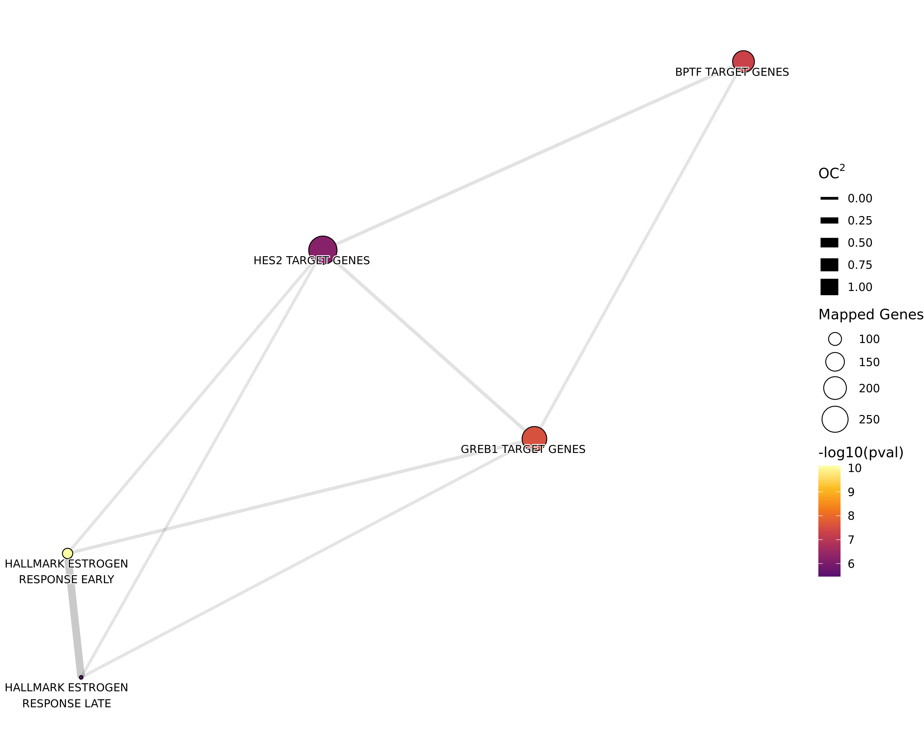
AR Up - H3K27ac Undetected
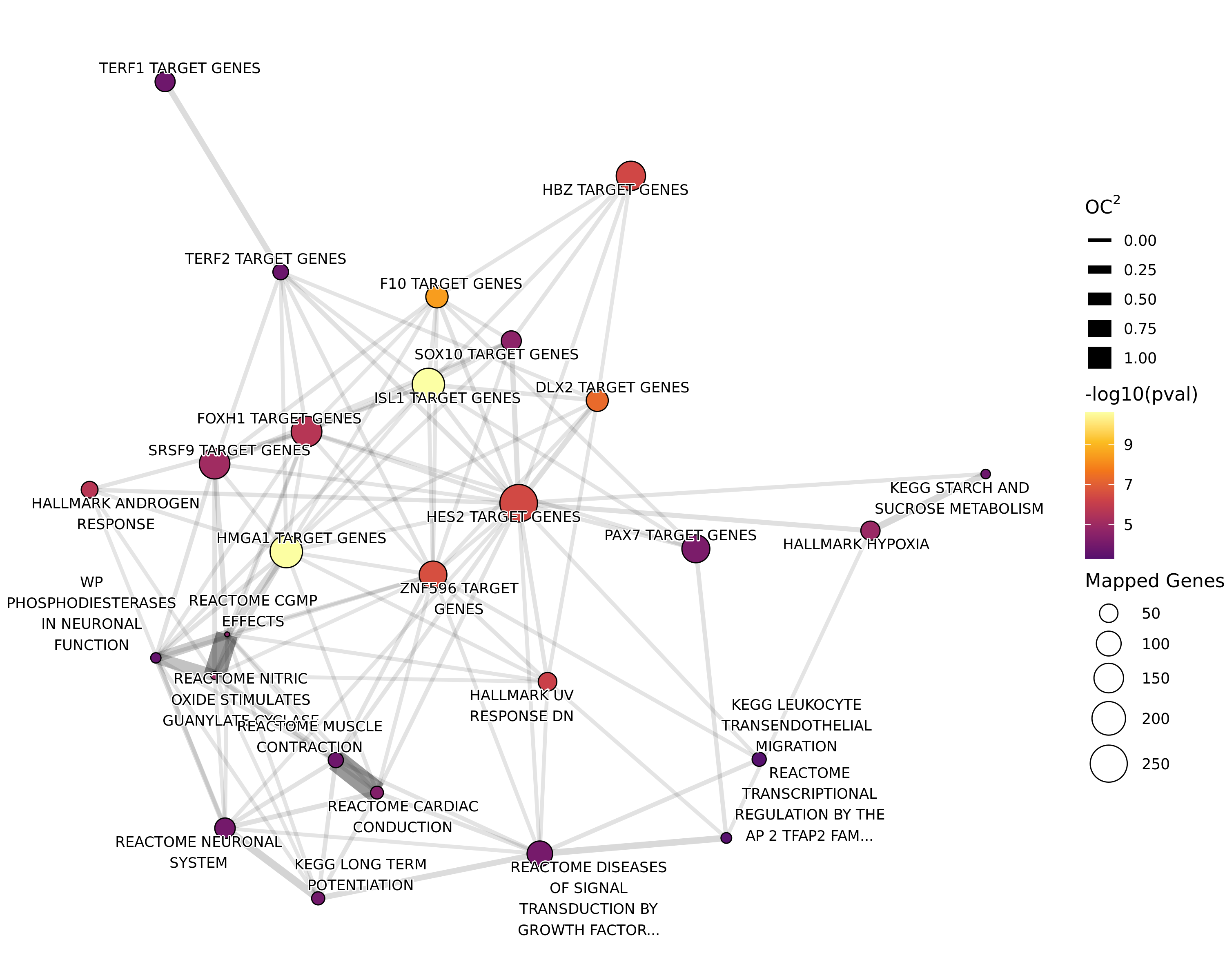
Comparison With RNA Seq
library(fgsea)
library(patchwork)
library(metap)
id2gene <- structure(gtf_gene$gene_name, names = gtf_gene$gene_id)
rna_status <- rnaseq %>%
  mutate(
    de_status = case_when(
      !!sym(rna_fdr_col) < fdr_alpha & !!sym(rna_lfc_col) < 0 ~ "Down",
      !!sym(rna_fdr_col) < fdr_alpha & !!sym(rna_lfc_col) > 0 ~ "Up",
      !!sym(rna_fdr_col) >= fdr_alpha ~ "Unchanged"
    )
  ) %>%
  dplyr::select(gene_id, gene_name, de_status) %>%
  bind_rows(
    gtf_gene %>%
      subset(!gene_id %in% rnaseq$gene_id) %>%
      select(gene_id, gene_name) %>%
      mcols() %>%
      as_tibble() %>%
      mutate(de_status = "Undetected")
  ) %>%
  mutate(
    de_status = factor(
      de_status, levels = str_to_title(names(colours$direction))
    )
  ) %>%
  arrange(gene_id)
rna_p_col <- colnames(rnaseq)[
  str_detect(str_to_lower(colnames(rnaseq)), "pval|p\\.val")
][1]
stopifnot(length(rna_p_col) == 1)
ids_by_group <- all_windows %>%
  as_tibble() %>%
  mutate(
    r1 = rank(!!sym(glue("{c1}_fdr")), ties.method = "min"),
    r2 = rank(!!sym(glue("{c2}_fdr")), ties.method = "min")
  ) %>%
  arrange(r1 + r2) %>%
  dplyr::select(gene_id, status, r1, r2) %>%
  unnest(everything()) %>%
  distinct(gene_id, .keep_all = TRUE) %>%
  droplevels() %>%
  split(.$status) %>%
  lapply(pull, "gene_id")
any_de <- sum(rnaseq[[rna_fdr_col]] < fdr_alpha) > 0
Volcano Plots
ids_by_group %>%
  lapply(function(x) tibble(gene_id = x)) %>%
  bind_rows(.id = "binding_status") %>%
  mutate(
    binding_status = factor(binding_status, levels = combs) %>%
      fct_lump_prop(0.01)
  ) %>%
  full_join(rnaseq, by = "gene_id") %>%
  dplyr::filter(!is.na(gene_name)) %>%
  mutate(
    binding_status = fct_na_value_to_level(binding_status, level = "No Targets"),
    de_status = case_when(
      DE & !!sym(rna_lfc_col) > 0 ~ "Up",
      DE & !!sym(rna_lfc_col) < 0 ~ "Down",
      TRUE ~ "Unchanged"
    ) %>%
      factor(levels = c("Up", "Down", "Unchanged"))
  ) %>%
  ggplot(
    aes(!!sym(rna_lfc_col), -log10(!!sym(rna_p_col)), colour = de_status)
  ) +
  geom_point() +
  geom_text_repel(
    aes(label = gene_name),
    data = . %>%
      arrange(!!sym(rna_p_col)) %>%
      dplyr::filter(DE) %>%
      split(.$binding_status) %>%
      lapply(dplyr::slice, 1:2) %>%
      bind_rows(),
    show.legend = FALSE
  ) +
  geom_text(
    aes(label = lab),
    data = . %>%
      group_by(binding_status) %>%
      summarise(n = dplyr::n()) %>%
      mutate(lab = glue("n = {comma(n)}")),
    x = min(rnaseq[[rna_lfc_col]]) + 0.9 * diff(range(rnaseq[[rna_lfc_col]])),
    y = 1,
    colour = "black",
    inherit.aes = FALSE,
    show.legend = FALSE
  ) +
  facet_wrap(~binding_status) +
  scale_colour_manual(
    values = colours$direction[c("up", "down", "unchanged")] %>%
      unlist() %>%
      setNames(str_to_title(names(.)))
  ) +
  labs(colour = "DE Status") +
  theme(legend.position = "right")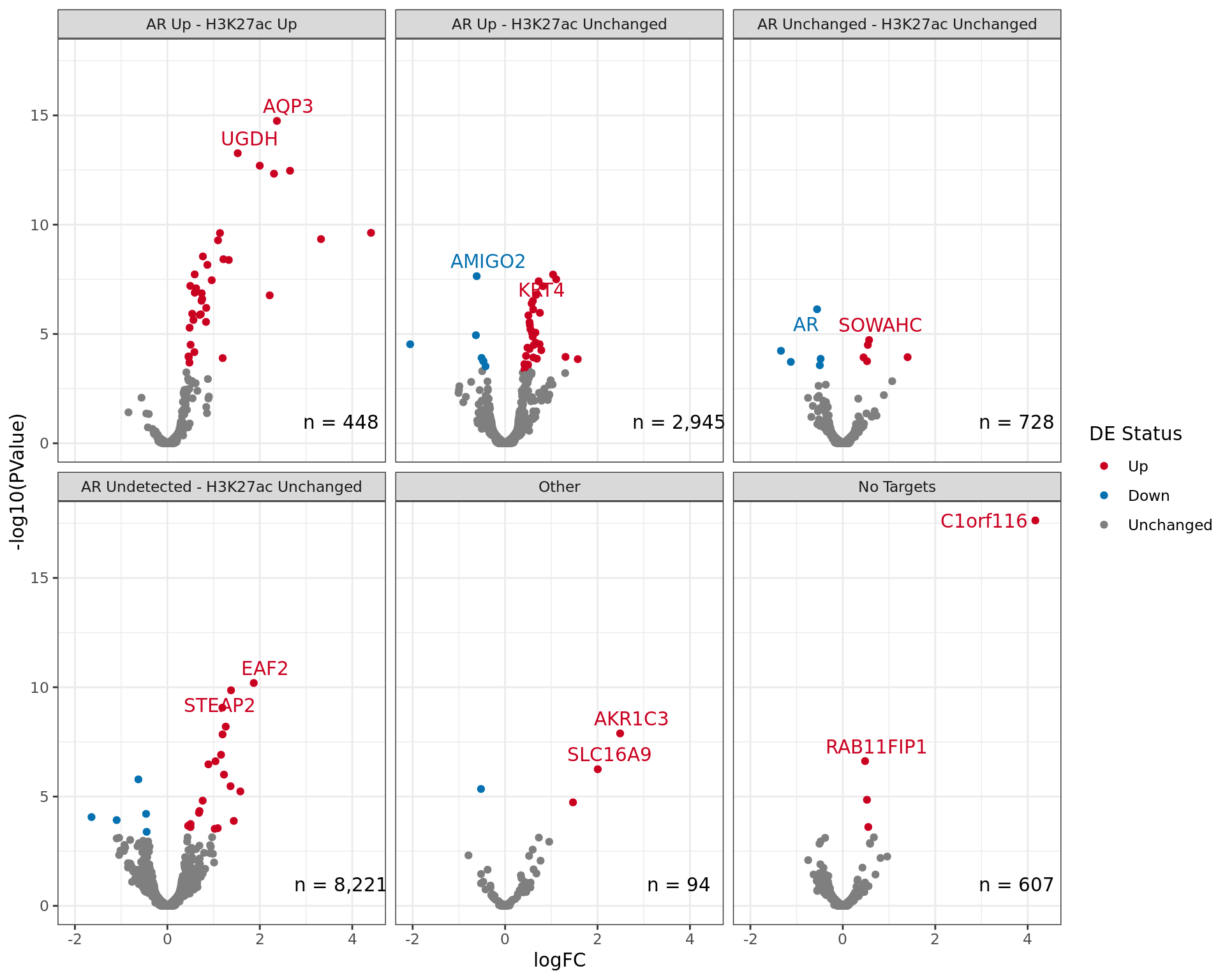
Volcano plots for differential expression separated by target binding patterns. Some genes will have multiple target binding regions mapped to them, and may appear in multiple panels. The two most highly ranked genes for differential expression are labelled in each panel. All DE genes are listed with full binding patterns in the table below.
DE Genes And Pairwise Binding
col_defs <- list2(
  de = colDef(
    name = "Gene", maxWidth = 120
  ),
  logFC = colDef(
    name = "logFC<br>(RNA-Seq)",
    html = TRUE,
    aggregate = "mean",
    maxWidth = 100,
    format = colFormat(digits = 2),
    style = JS(
      glue(
        "function(rowInfo) {
              var value = rowInfo.row['logFC']
              if (value < 0) {
                var color = '{{colours$direction[['down']]}}'
              } else if (value > 0) {
                var color = '{{colours$direction[['up']]}}'
              }
              return { color: color }
            }",
        .open = "{{", .close = "}}"
      )
    )
  ),
  range = colDef(
    name = "Range",
    aggregate = JS(
      "function(values){
              var chrom = [];
              var rng = [];
              var start = [];
              var end = [];
              for (i = 0; i < values.length; i++) {
                chrom[i] = values[i].split(':')[0];
                rng[i] = values[i].split(':')[1];
                start[i] = rng[i].split('-')[0];
                end[i] = rng[i].split('-')[1];
              }

              min_start = Math.min(...start);
              max_end = Math.max(...end);
              var ret_val = [...new Set(chrom)] + ':' + min_start.toString() + '-' + max_end.toString();

              return ret_val

            }"
    )
  ),
  region = colDef(
    aggregate = "unique",
    name = "Region"
  ),
  "{c1}_logFC" := colDef(
    name = comps[[1]],
    maxWidth = 100,
    format = colFormat(digits = 2),
    style = function(value) {
      cl <- ifelse(
        value > 0, colours$direction[["up"]], colours$direction[["down"]]
      )
      list(color = cl)
    }
  ),
  "{c2}_logFC" := colDef(
    name = comps[[2]],
    maxWidth = 100,
    format = colFormat(digits = 2),
    style = function(value) {
      cl <- ifelse(
        value > 0, colours$direction[["up"]], colours$direction[["down"]]
      )
      list(color = cl)
    }
  ),
  "{c1}_status" := colDef(
    aggregate = "unique",
    name = comps[[1]],
    maxWidth = 150
  ),
  "{c2}_status" := colDef(
    aggregate = "unique",
    name = comps[[2]],
    maxWidth = 150
  )
)
if (has_features) col_defs$feature <- colDef(
  name = "Feature",
  aggregate = "unique"
)
htmltools::tags$caption(
  htmltools::em(
    glue(
    "
    All differentially expressed genes where binding was detected in both
    comparisons.
    "
    )
  )
)de_genes_both_comps <- all_windows %>%
as_tibble() %>%
dplyr::select(
any_of(c("range", "region", "feature")), ends_with("logFC"), ends_with("status"),
any_of(c("detected"))
) %>%
mutate(
de = lapply(detected, intersect, dplyr::filter(rnaseq, !!sym(rna_fdr_col) < fdr_alpha)$gene_name)
) %>%
dplyr::filter(
vapply(de, length, integer(1)) > 0,
str_detect(status, "Up|Down"),
!str_detect(status, "Undetected")
) %>%
unnest(de) %>%
left_join(rnaseq, by = c("de" = "gene_name")) %>%
mutate(direction = ifelse(logFC > 0, "Up", "Down")) %>%
droplevels() %>%
dplyr::select(
de, logFC, any_of(c("range", "region", "feature")), ends_with("logFC"),
ends_with("_status")
)
de_genes_both_comps %>%
reactable(
filterable = TRUE, resizable = TRUE, showPageSizeOptions = TRUE,
groupBy = "de",
columns = col_defs,
columnGroups = list(
colGroup(
name = "ChIP logFC",
columns = as.character(glue("{comps}_logFC"))
),
colGroup(
name = "ChIP Status",
columns = as.character(glue("{comps}_status"))
)
),
theme = reactableTheme(style = list(fontSize = 14))
)Binding Pattern GSEA
rna_dir_ranks <- rnaseq %>%
  mutate(
    ranking_stat = -sign(!!sym(rna_lfc_col))*log10(!!sym(rna_p_col)) %>%
      setNames(gene_id)
  ) %>%
  arrange(ranking_stat) %>%
  dplyr::filter(!!sym(rna_p_col) < 1) %>%
  pull("ranking_stat")
rna_sig_ranks <- rna_dir_ranks %>%
  abs() %>%
  sort()
status_gs <- all_windows %>%
  select(status, starts_with("gene")) %>%
  as_tibble() %>%
  split(.$status) %>%
  lapply(pull, "gene_id") %>%
  lapply(unlist) %>%
  lapply(unique) %>%
  .[vapply(., length, integer(1)) > min_gs_size]
GSEA analysis was performed taking the set of genes mapped to each binding pattern. This was initially performed ranking the RNA-Seq results in order of significance, with most significantly up-regulated and one end and the most significantly down-regulated at the other, i.e. Directional GSEA A secondary analysis was performed taking only statistical significance into account, without including the direction of any change in expression, i.e. Non_Directional GSEA. This second analysis allows for detecting regulatory changes due to altered binding, but which are spread between both up- and down-regulation, as may be induced by the presence of other co-factors not under direct investigation here.
Directional GSEA
gsea_dir <- fgsea(status_gs, rna_dir_ranks) %>%
  as_tibble() %>%
  arrange(pval) %>%
  mutate(padj = p.adjust(pval, adj_method)) %>%
  as_tibble()
p <- gsea_dir %>%
  dplyr::filter(padj < enrich_alpha, size >= min_sig) %>%
  pull("pathway") %>%
  lapply(
    function(x) {
      plotEnrichment(status_gs[[x]], rna_dir_ranks) +
        ggtitle(x) +
        theme(
          plot.title = element_text(hjust = 0.5, size = 10)
        )
    }
  )
cp <- htmltools::em(
glue(
"Combined windows were mapped to genes, and their position amongst the ",
"RNA-Seq results was assessed. {sum(gsea_dir$padj < enrich_alpha)} sets of windows were ",
"associated with changes in gene expression, using the sign of ",
"fold-change and ranking statistic to initially rank the ",
"{comma(nrow(rnaseq), 1)} genes considered as detected."
)
)
tbl <- gsea_dir %>%
mutate(
`Edge Size` = vapply(leadingEdge, length, integer(1)),
leadingEdge = lapply(leadingEdge, function(x) id2gene[x]) %>%
vapply(paste, character(1), collapse = "; "),
Direction = ifelse(NES > 0, "\u21E7 Up-regulated", "\u21E9 Down-regulated")
) %>%
separate(pathway, comps, sep = " - ") %>%
dplyr::select(
all_of(comps), Windows = size, Direction,
p = pval, padj, `Edge Size`, `Leading Edge` = leadingEdge
) %>%
reactable(
filterable = TRUE,
columns = list2(
"{comps[[1]]}" := colDef(
maxWidth = 150,
cell = function(value) {
html_symbol <- ""
if (str_detect(value, "Up")) html_symbol <- "\u21E7"
if (str_detect(value, "Down")) html_symbol <- "\u21E9"
paste(html_symbol, value)
},
style = function(value) {
colour <- case_when(
str_detect(value, "Up") ~ colours$direction[["up"]],
str_detect(value, "Down") ~ colours$direction[["down"]],
TRUE ~ colours$direction[["unchanged"]]
)
list(color = colour)
}
),
"{comps[[2]]}" := colDef(
maxWidth = 150,
cell = function(value) {
html_symbol <- ""
if (str_detect(value, "Up")) html_symbol <- "\u21E7"
if (str_detect(value, "Down")) html_symbol <- "\u21E9"
paste(html_symbol, value)
},
style = function(value) {
colour <- case_when(
str_detect(value, "Up") ~ colours$direction[["up"]],
str_detect(value, "Down") ~ colours$direction[["down"]],
TRUE ~ colours$direction[["unchanged"]]
)
list(color = colour)
}
),
Windows = colDef(maxWidth = 80),
Direction = colDef(
name = "Gene Direction",
maxWidth = 120,
style = function(value) {
colour <- ifelse(
str_detect(value, "Up"),
colours$direction[["up"]],
colours$direction[["down"]]
)
list(color = colour)
},
),
p = colDef(
cell = function(value) ifelse(
value < 0.001,
sprintf("%.2e", value),
sprintf("%.3f", value)
),
maxWidth = 80
),
padj = colDef(
name = glue("p<sub>{adj_method}</sub>"), html = TRUE,
cell = function(value) {
ifelse(
value < 0.001, sprintf("%.2e", value), sprintf("%.3f", value)
)
}
),
"Edge Size" = colDef(maxWidth = 80),
"Leading Edge" = colDef(
minWidth = 150,
cell = function(value) with_tooltip(value, width = 50)
)
)
)
div(class = "table",
div(class = "table-header",
div(class = "caption", cp),
tbl
)
)wrap_plots(p)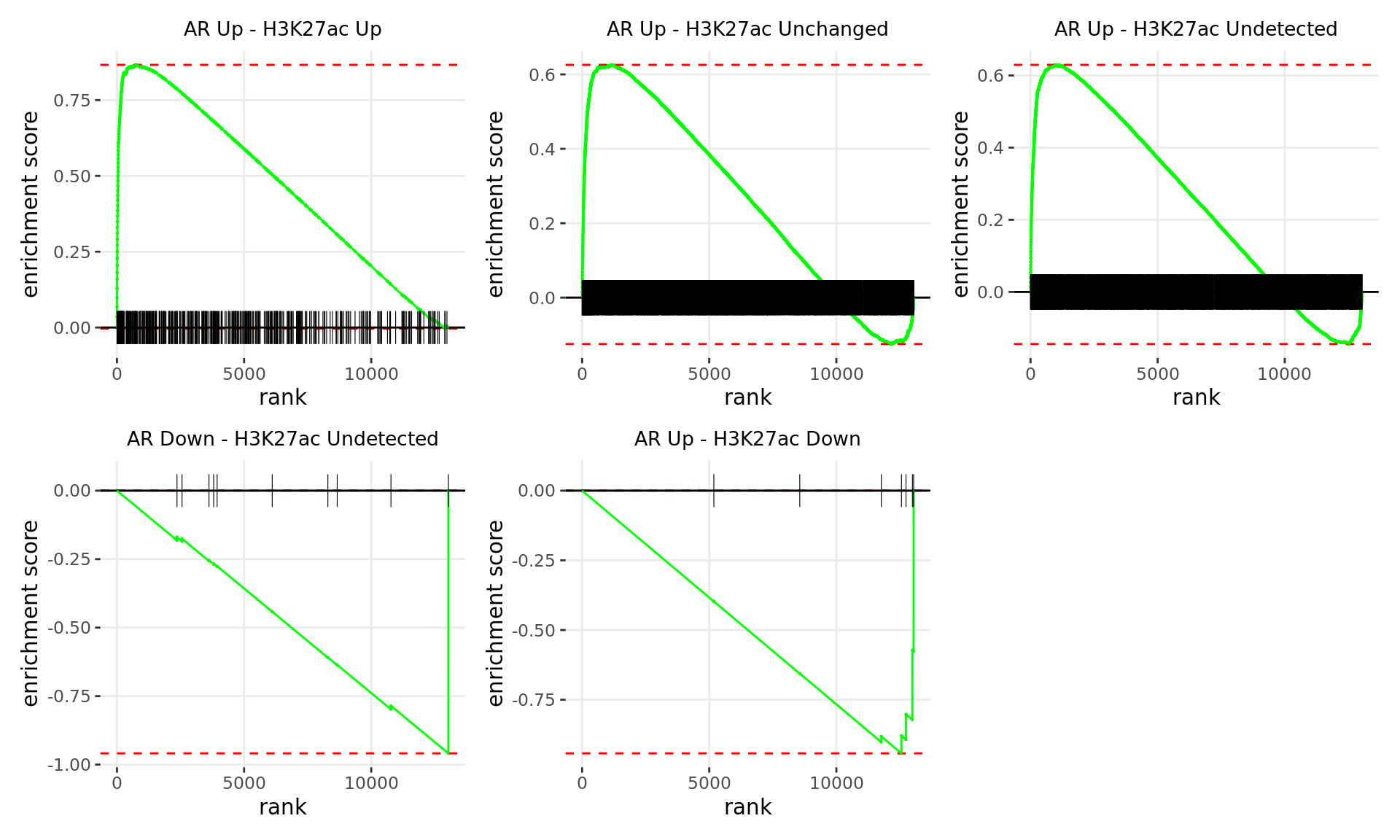
Barcode plots for the top 5 sets of windows associated with directional changes in gene expression.
Non-Directional GSEA
gsea_nondir <- suppressWarnings(
  fgsea(status_gs, rna_sig_ranks, scoreType = "pos")
) %>%
  as_tibble() %>%
  arrange(pval) %>%
  mutate(padj = p.adjust(pval, adj_method))
p <- gsea_nondir %>%
  dplyr::filter(padj < enrich_alpha, size >= min_sig) %>%
  pull("pathway") %>%
  lapply(
    function(x) {
      plotEnrichment(status_gs[[x]], rna_sig_ranks) +
        ggtitle(x) +
        theme(plot.title = element_text(hjust = 0.5, size = 10))
    }
  )
txt <- ifelse(
  length(p) > 0,
  glue(""),
  glue("No association was found between changed binding across {comps[[1]]} and {comps[[2]]} when combined with *overall* significance in differentially expressed genes.")
)
cp <- htmltools::em(
glue(
"Combined windows were mapped to genes, and their position amongst the ",
"RNA-Seq results was assessed. {sum(gsea_nondir$padj < enrich_alpha)} sets of windows were ",
"associated with changes in gene expression, using only the p-value to ",
"rank the {comma(nrow(rnaseq), 1)} genes considered as detected."
)
)
tbl <- gsea_nondir %>%
mutate(
`Edge Size` = vapply(leadingEdge, length, integer(1)),
leadingEdge = lapply(leadingEdge, function(x) id2gene[x]) %>%
vapply(paste, character(1), collapse = "; ")
) %>%
separate(pathway, comps, sep = " - ") %>%
dplyr::select(
all_of(comps), Windows = size,
p = pval, padj, `Edge Size`, `Leading Edge` = leadingEdge
) %>%
reactable(
filterable = TRUE,
columns = list2(
"{comps[[1]]}" := colDef(
maxWidth = 150,
cell = function(value) {
html_symbol <- ""
if (str_detect(value, "Up")) html_symbol <- "\u21E7"
if (str_detect(value, "Down")) html_symbol <- "\u21E9"
paste(html_symbol, value)
},
style = function(value) {
colour <- case_when(
str_detect(value, "Up") ~ colours$direction[["up"]],
str_detect(value, "Down") ~ colours$direction[["down"]],
TRUE ~ colours$direction[["unchanged"]]
)
list(color = colour)
}
),
"{comps[[2]]}" := colDef(
maxWidth = 150,
cell = function(value) {
html_symbol <- ""
if (str_detect(value, "Up")) html_symbol <- "\u21E7"
if (str_detect(value, "Down")) html_symbol <- "\u21E9"
paste(html_symbol, value)
},
style = function(value) {
colour <- case_when(
str_detect(value, "Up") ~ colours$direction[["up"]],
str_detect(value, "Down") ~ colours$direction[["down"]],
TRUE ~ colours$direction[["unchanged"]]
)
list(color = colour)
}
),
Windows = colDef(maxWidth = 80),
p = colDef(
cell = function(value) ifelse(
value < 0.001,
sprintf("%.2e", value),
sprintf("%.3f", value)
),
maxWidth = 80
),
padj = colDef(
name = glue("p<sub>{adj_method}</sub>"), html = TRUE,
cell = function(value) {
ifelse(
value < 0.001, sprintf("%.2e", value), sprintf("%.3f", value)
)
}
),
"Edge Size" = colDef(maxWidth = 80),
"Leading Edge" = colDef(
minWidth = 150,
cell = function(value) with_tooltip(value, width = 50)
)
)
)
div(class = "table",
div(class = "table-header",
div(class = "caption", cp),
tbl
)
)wrap_plots(p)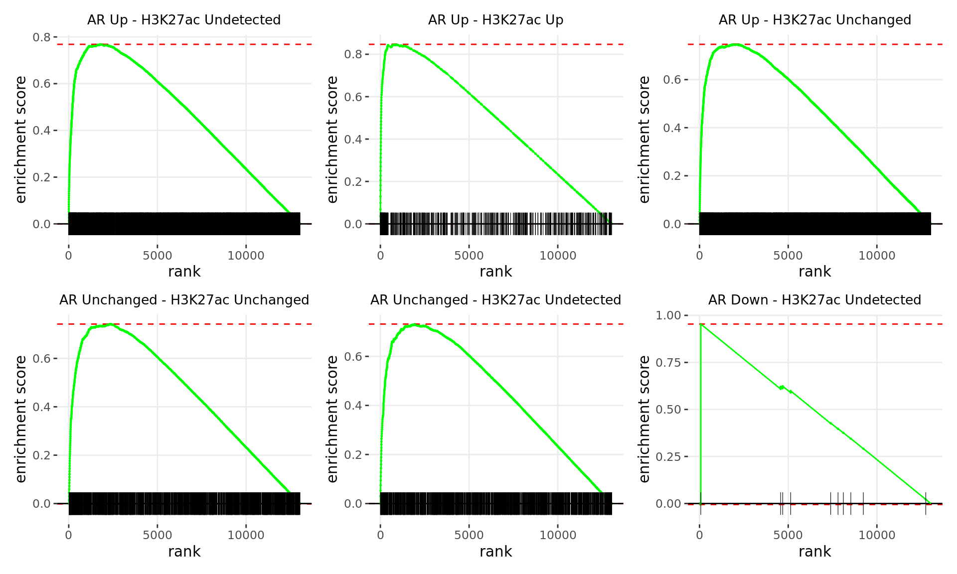
Barcode plots for the top 6 sets of windows associated with non-directional changes in gene expression.
Integration of RNA and ChIP Enrichment Analyses
Directional GSEA was performed on the set of RNA-Seq results and given that enrichment for differentially bound target is an orthogonal measure, enrichment for a set of potential pathways for each pairwise set of regions was performed. The p-values from binding enrichment and GSEA were combined using Wilkinson’s method for meta-analysis, taking the maximum p-value and adjusting the resulting p-value using the same strategy as earlier. Any pathways are annotated as being significant in both, either or neither dataset when being analysed individually.
Distances between nodes (gene-sets) for any network plots were estimated by using the similarity of genes within the leading edge which were also mapped to binding regions showing the respective pattern. If the genes of interest from any two pathways were identical, only the most highly-ranked pathway was included in the network, and similarly if one gene-set was a subset of another, the most highly-ranked was retained for visualisation.
rnaseq_gsea <- suppressWarnings(
  fgsea(
    pathways = gs_by_gsid,
    stats = rna_dir_ranks,
    minSize = min_gs_size,
    maxSize = max_gs_size
  )
) %>%
  dplyr::filter(!is.na(pval))
status_cols <- setNames(
  hcl.colors(4, "Viridis", rev = TRUE),
  c("Both", "ChIP Only", "RNA Only", "Neither")
)
cmn_res <- goseq_group_res %>%
  lapply(dplyr::select, group, gs_name, pval_goseq = pval, adj_p, starts_with("num")) %>%
  lapply(
    left_join,
    dplyr::select(rnaseq_gsea, gs_name = pathway, NES, pval_gsea = pval, padj, leadingEdge),
    by = "gs_name"
  ) %>%
  lapply(
    nest, p = starts_with("pval")
  ) %>%
  lapply(
    dplyr::rename, padj_chip = adj_p, padj_rna = padj
  ) %>%
  lapply(
    mutate,
    pval = vapply(
      p, function(x) metap::maximump(unlist(x))$p, numeric(1)
    ),
    adj_p = p.adjust(pval, adj_method)
  ) %>%
  lapply(dplyr::filter, adj_p < enrich_alpha) %>%
  lapply(
    mutate,
    status = case_when(
      padj_chip < enrich_alpha & padj_rna < enrich_alpha ~ "Both",
      !padj_chip < enrich_alpha & padj_rna < enrich_alpha ~ "RNA Only",
      padj_chip < enrich_alpha & !padj_rna < enrich_alpha ~ "ChIP Only",
      !padj_chip < enrich_alpha & !padj_rna < enrich_alpha ~ "Neither"
    ) %>%
      factor(levels = names(status_cols)),
    leadingEdge = lapply(leadingEdge, intersect, group_ids[[unique(group)]]),
    numDEInCat = vapply(leadingEdge, length, integer(1)),
    genes = vapply(
      leadingEdge, function(x) paste(id2gene[x], collapse = "; "), character(1)
    )
  ) %>%
  lapply(dplyr::filter, numDEInCat >= min_sig) %>%
  lapply(
    select,
    group, gs_name, adj_p, NES, status, starts_with("padj"),
    starts_with("num"), leadingEdge, genes
  ) %>%
  lapply(dplyr::filter, numDEInCat > 0) %>%
  .[vapply(., nrow, integer(1)) > 0]
tg_cmn <- names(cmn_res) %>%
  lapply(
    function(x) {
      make_tbl_graph(
        cmn_res[[x]],
        setNames(cmn_res[[x]]$leadingEdge, cmn_res[[x]]$gs_name)
      )
    }
  ) %>%
  setNames(names(cmn_res)) %>%
  .[vapply(., length, integer(1)) >= min_network_size]
any_sig <- length(cmn_res) > 0
plot_net <- length(tg_cmn) > 0
txt <- ifelse(any_sig, "### Results {.tabset}", "No shared enrichment was found")
Results
htmltools::tagList(
  names(cmn_res) %>%
    lapply(
      function(x) {
        df <- cmn_res[[x]] %>%
          dplyr::select(
            gs_name, adj_p, NES, status, starts_with("padj"), numDEInCat, genes
          )
        tbl <- df %>%
          arrange(adj_p) %>%
          reactable(
            filterable = TRUE, showPageSizeOptions = TRUE,
            columns = list(
              gs_name = colDef(
                name = "Gene Set",
                cell = function(value) htmltools::tags$a(
                  href = gs_url[[value]],
                  target = "_blank",
                  str_replace_all(value, "_", " ")
                ),
                minWidth = 120
              ),
              NES = colDef(
                format = colFormat(digits = 2),
                style = function(value) {
                  col <- ifelse(value > 0, colours$direction$up, colours$direction$down)
                  list(color = col)
                },
                maxWidth = 80
              ),
              adj_p = colDef(
                name = "p<sub>adj</sub>", html = TRUE,
                cell = function(value) ifelse(
                  value < 0.001,
                  sprintf("%.2e", value),
                  sprintf("%.3f", value)
                ),
                maxWidth = 80
              ),
              status = colDef(name = "Individual Status", maxWidth = 100),
              padj_rna = colDef(
                name =  glue("p<sub>{extra_params$enrichment$adj}</sub> (RNA)"), html = TRUE,
                cell = function(value) ifelse(
                  value < 0.001,
                  sprintf("%.2e", value),
                  sprintf("%.3f", value)
                ),
                maxWidth = 80
              ),
              padj_chip = colDef(
                name =  glue("p<sub>{extra_params$enrichment$adj}</sub> (ChIP)"), html = TRUE,
                cell = function(value) ifelse(
                  value < 0.001,
                  sprintf("%.2e", value),
                  sprintf("%.3f", value)
                ),
                maxWidth = 80
              ),
              numDEInCat = colDef(name = "# Targets in Leading Edge", maxWidth = 100),
              genes = colDef(
                name = "Targets in Leading Edge",
                cell = function(value) with_tooltip(value, width = 50)
              )
            )
          )
        cp <- glue(
          "The {nrow(df)} Gene sets considered significant when combining GSEA
          from RNA-Seq and enrichment anaylsis from binding sites corresponding
          to {x}. The direction of the NES indicates the enriched direction in
          the RNA-Seq data.
        "
        )
        htmltools::div(
          htmltools::div(
            id = x %>%
              str_to_lower %>%
              str_replace_all(" ", "-") %>%
              str_replace_all("-+", "-") %>%
              paste("gsea", sep = "-"),
            class = "section level4",
            htmltools::h4(class = "tabset", x),
            htmltools::tags$em(cp),
            tbl
          )
        )
      }
    ) %>%
    setNames(names(cmn_res))
)
AR Up - H3K27ac Unchanged
The 7 Gene sets considered significant when combining GSEA from RNA-Seq and enrichment anaylsis from binding sites corresponding to AR Up - H3K27ac Unchanged. The direction of the NES indicates the enriched direction in the RNA-Seq data.AR Up - H3K27ac Undetected
The 5 Gene sets considered significant when combining GSEA from RNA-Seq and enrichment anaylsis from binding sites corresponding to AR Up - H3K27ac Undetected. The direction of the NES indicates the enriched direction in the RNA-Seq data.AR Up - H3K27ac Up
The 16 Gene sets considered significant when combining GSEA from RNA-Seq and enrichment anaylsis from binding sites corresponding to AR Up - H3K27ac Up. The direction of the NES indicates the enriched direction in the RNA-Seq data.All Groups
cmn_res %>%
  bind_rows() %>%
  arrange(adj_p) %>%
  left_join(n_mapped, by = c("group" = "status")) %>%
  mutate(
    gs_name = fct_inorder(gs_name) %>%
      fct_relabel(str_replace_all, "_", " ") %>%
      fct_relabel(str_trunc, width = 60),
    prop = numDEInCat / mapped,
    group = factor(group, levels = arrange(n_mapped, mapped)$status)
  ) %>%
  droplevels() %>%
  ggplot(aes(fct_rev(group), fct_rev(gs_name))) +
  geom_point(aes(size = prop, fill = -log10(adj_p)), shape = 21) +
  geom_ysidecol(
    aes(x = numInCat), data = . %>% distinct(gs_name, numInCat),
  ) +
  geom_xsidecol(
    aes(y = mapped),
    data = n_mapped %>%
      dplyr::filter(status %in% names(cmn_res)) %>%
      dplyr::rename(group = status),
    width = 0.5
  ) +
  scale_x_discrete(labels = label_wrap(10)) +
  scale_ysidex_continuous(expand = expansion(c(0, 0.15))) +
  scale_xsidey_continuous(
    expand = expansion(c(0, 0.15))
  ) +
  scale_fill_viridis_c(option = "inferno", begin = 0.2) +
  scale_size(range = c(0, 5), labels = percent) +
  labs(
    x = c(), y = c(), size = "% Mapped\n& Detected\nGenes",
    fill = expr(paste(-log[10], p[!!sym(adj_method)]))
  ) +
  theme(
    panel.grid = element_blank(),
    axis.text = element_text(size = 8),
    legend.position = "right",
    ggside.panel.scale.x = 0.2,
    ggside.panel.scale.y = 0.3,
    ggside.axis.text.x.bottom = element_text(angle = 270, hjust = 0, vjust = 0.5)
) 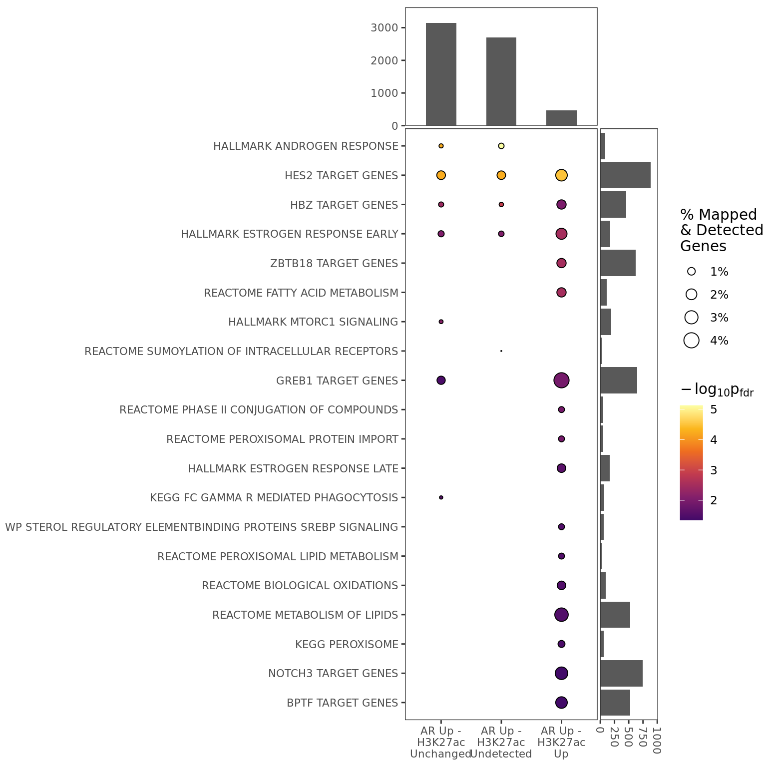
Combined enrichment across all groups, incorporating RNA expression data, showing only significant results for enrichment. The top panel shows how many detected genes were mapped to sites for each group, whilst the right panel shows gene set size, using detected genes only. Point sizes indicate the proportion of mapped and detected genes which are from each pathway.
Network Plots
htmltools::tagList(
  names(tg_cmn) %>%
    mclapply(
      function(x) {
        ## Export the image
        img_out <- file.path(
          fig_path,
          x %>%
            str_replace_all(" ", "_") %>%
            str_replace_all("_-_", "-") %>%
            paste0("_rnaseq_network.", fig_type)
        )
        fig_fun(
          filename = img_out,
          width = knitr::opts_current$get("fig.width"),
          height = knitr::opts_current$get("fig.height")
        )
        p <- tg_cmn[[x]] %>%
          activate(nodes) %>%
          mutate(direction = ifelse(NES > 0, "Up", "Down")) %>%
          ggraph(layout = net_layout, weights = oc^2) +
          geom_edge_link(aes(width = oc^2, alpha = oc^2)) +
          geom_node_point(
            aes(fill = status, size = numDEInCat),
            shape = 21
          ) +
          geom_node_text(
            aes(label = label, colour = direction),
            size = 3,
            data = . %>%
              mutate(
                label = str_replace_all(label, "_", " ") %>% str_trunc(60) %>% str_wrap(width = 18)
              ),
            repel = TRUE,
            max.overlaps = max(10, round(length(tg_cmn[[x]]) / 4, 0)),
            bg.color = "white", bg.r = 0.1
          ) +
          scale_x_continuous(expand = expansion(c(0.1, 0.1))) +
          scale_y_continuous(expand = expansion(c(0.1, 0.1))) +
          scale_fill_manual(values = status_cols) +
          scale_size_continuous(range = c(1, 10)) +
          scale_edge_width(range = c(1, 6), limits = c(0, 1)) +
          scale_edge_alpha(range = c(0.1, 0.4), limits = c(0, 1)) +
          scale_colour_manual(
            values = setNames(
              unlist(colours$direction),
              str_to_title(names( unlist(colours$direction)))
            )
          ) +
          guides(edge_alpha = "none", edge_width = "none") +
          labs(
            size = "Targets In\nLeading Edge",
            colour = "GSEA\nDirection",
            fill = "Prior\nStatus",
          ) +
          theme_void()
        print(p)
        dev.off()
        ## Create html tags
        fig_link <- str_extract(img_out, "assets.+")
        cp <- htmltools::tags$em(
          glue(
            "
            Network plot showing enriched pathways mapped to genes
            associated with {x} in combination with GSEA results from
            the RNA-Seq data.
            "
          )
        )
        htmltools::div(
          htmltools::div(
            id = img_out %>%
              basename() %>%
              str_remove_all(glue(".{fig_type}$")) %>%
              str_to_lower() %>%
              str_replace_all("_", "-"),
            class = "section level4",
            htmltools::h4(x),
            htmltools::div(
              class = "figure", style = "text-align: center",
              htmltools::img(src = fig_link, width = "100%"),
              htmltools::tags$caption(cp)
            )
          )
        )
      },
      mc.cores = threads
    )
)
AR Up - H3K27ac Unchanged
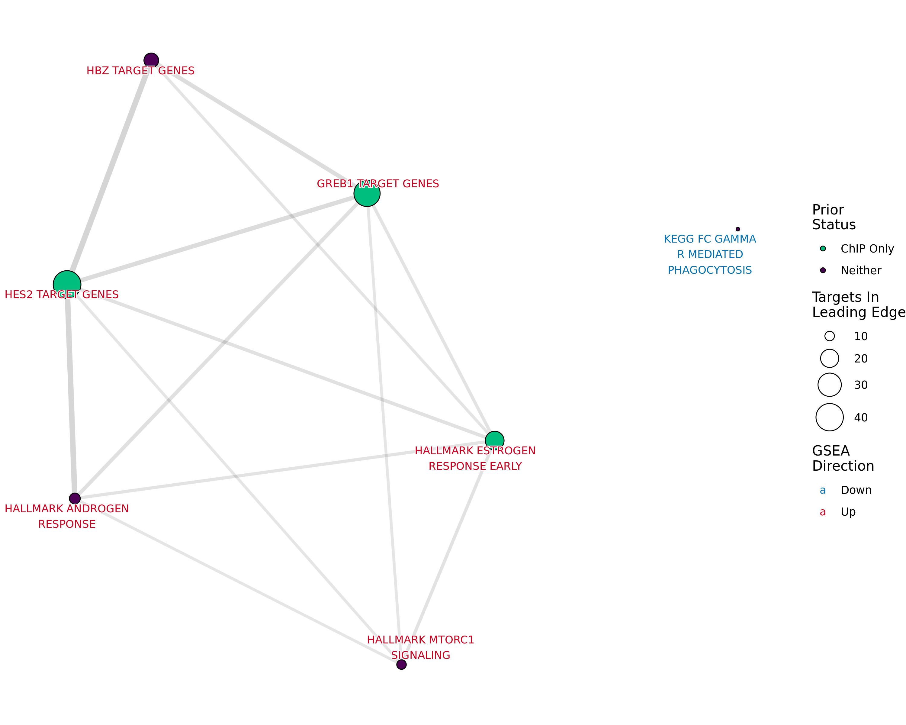
AR Up - H3K27ac Undetected
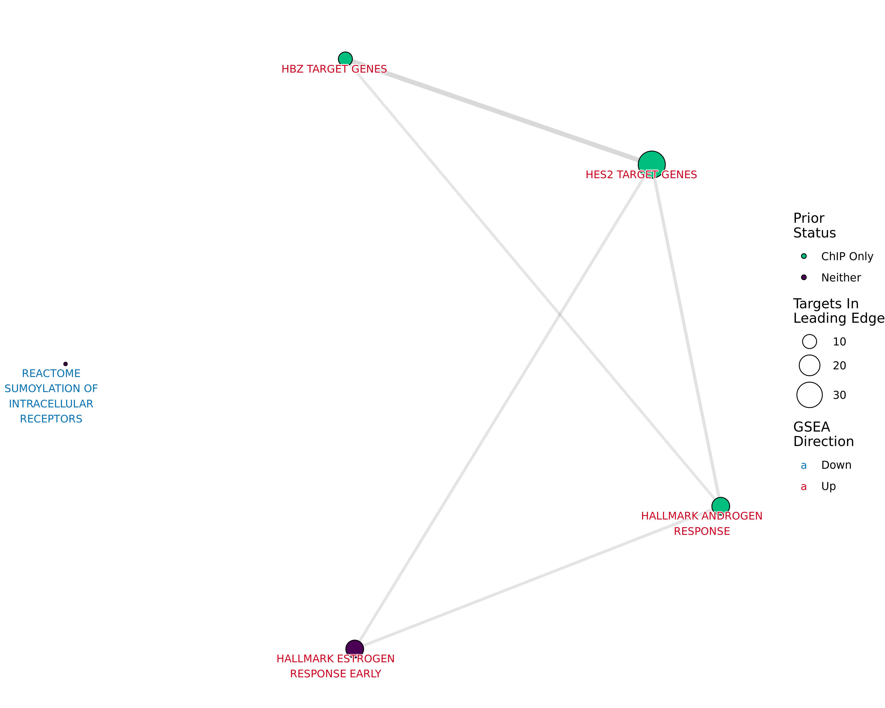
AR Up - H3K27ac Up
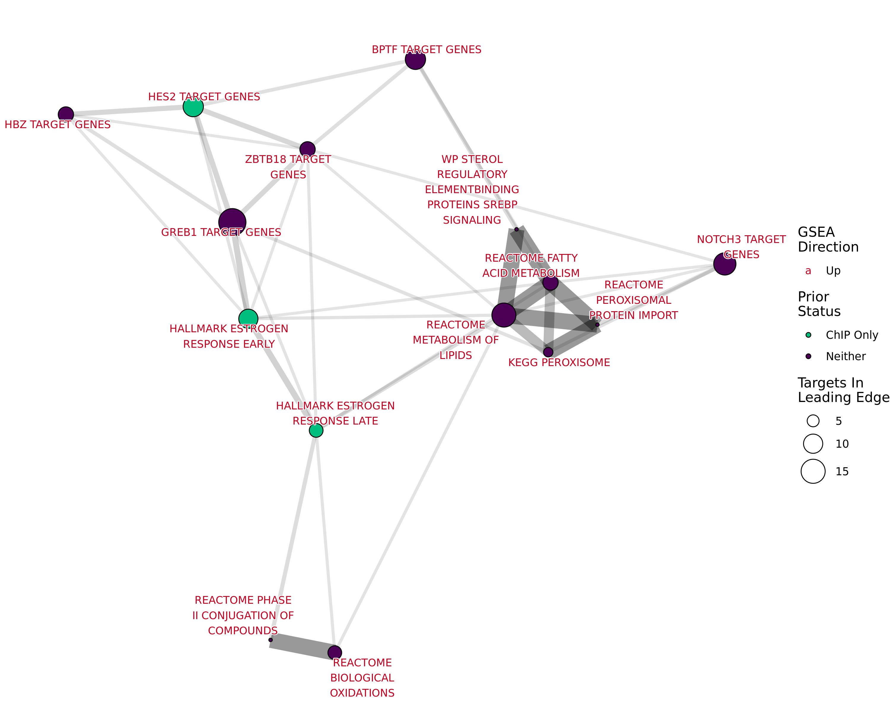
Data Export
write_rds(all_windows, all_out$results, compress = "gz")
save.image(all_out$renv)
all_windows %>%
as_tibble() %>%
dplyr::select(-detected) %>%
unnest(all_of("gene_id")) %>% # This ensures correct id2gene mappings
mutate(gene_name = id2gene[gene_id]) %>%
dplyr::select(
starts_with("gene"), range, any_of(c("region", "feature", "hic")),
) %>%
write_csv(
gzfile(all_out$csv)
)
write_csv(de_genes_both_comps, all_out$de_genes)
goseq_group_sig %>%
bind_rows() %>%
write_csv(all_out$goseq)
cmn_res %>%
bind_rows() %>%
mutate(
leadingEdge = vapply(leadingEdge, paste, character(1), collapse = "; "),
gs_url = gs_url[gs_name]
) %>%
write_csv(all_out$rna_enrichment)During this workflow, the following files were exported:
- csv: output/pairwise_comparisons/AR_H3K27ac/AR_E2_E2DHT-H3K27ac_E2_E2DHT-pairwise_comparison.csv.gz
- de_genes: output/pairwise_comparisons/AR_H3K27ac/AR_E2_E2DHT-H3K27ac_E2_E2DHT-de_genes.csv
- goseq: output/pairwise_comparisons/AR_H3K27ac/AR_E2_E2DHT-H3K27ac_E2_E2DHT-enrichment.csv
- results: output/pairwise_comparisons/AR_H3K27ac/AR_E2_E2DHT-H3K27ac_E2_E2DHT-all_windows.rds
- rna_enrichment: output/pairwise_comparisons/AR_H3K27ac/AR_E2_E2DHT-H3K27ac_E2_E2DHT-rnaseq_enrichment.csv
- renv: output/envs/AR_E2_E2DHT-H3K27ac_E2_E2DHT-pairwise_comparison.RData
References
R version 4.2.3 (2023-03-15)
Platform: x86_64-conda-linux-gnu (64-bit)
locale: LC_CTYPE=en_AU.UTF-8, LC_NUMERIC=C, LC_TIME=en_AU.UTF-8, LC_COLLATE=en_AU.UTF-8, LC_MONETARY=en_AU.UTF-8, LC_MESSAGES=en_AU.UTF-8, LC_PAPER=en_AU.UTF-8, LC_NAME=C, LC_ADDRESS=C, LC_TELEPHONE=C, LC_MEASUREMENT=en_AU.UTF-8 and LC_IDENTIFICATION=C
attached base packages: parallel, grid, stats4, stats, graphics, grDevices, utils, datasets, methods and base
other attached packages: metap(v.1.1), patchwork(v.1.1.2), fgsea(v.1.24.0), tidygraph(v.1.2.3), ggraph(v.2.1.0), extraChIPs(v.1.5.7), BiocParallel(v.1.32.5), GenomicInteractions(v.1.32.0), InteractionSet(v.1.26.0), SummarizedExperiment(v.1.28.0), Biobase(v.2.58.0), MatrixGenerics(v.1.10.0), matrixStats(v.1.0.0), goseq(v.1.50.0), geneLenDataBase(v.1.34.0), BiasedUrn(v.2.0.10), htmltools(v.0.5.5), msigdbr(v.7.5.1), ggside(v.0.2.2), rlang(v.1.1.1), ggrepel(v.0.9.3), scales(v.1.2.1), magrittr(v.2.0.3), ComplexUpset(v.1.3.3), VennDiagram(v.1.7.3), futile.logger(v.1.4.3), rtracklayer(v.1.58.0), plyranges(v.1.18.0), GenomicRanges(v.1.50.0), GenomeInfoDb(v.1.34.9), IRanges(v.2.32.0), S4Vectors(v.0.36.0), BiocGenerics(v.0.44.0), reactable(v.0.4.4), yaml(v.2.3.7), pander(v.0.6.5), glue(v.1.6.2), lubridate(v.1.9.2), forcats(v.1.0.0), stringr(v.1.5.0), dplyr(v.1.1.2), purrr(v.1.0.1), readr(v.2.1.4), tidyr(v.1.3.0), tibble(v.3.2.1), ggplot2(v.3.4.2) and tidyverse(v.2.0.0)
loaded via a namespace (and not attached): utf8(v.1.2.3), tidyselect(v.1.2.0), RSQLite(v.2.3.1), AnnotationDbi(v.1.60.0), htmlwidgets(v.1.6.2), munsell(v.0.5.0), codetools(v.0.2-19), interp(v.1.1-4), withr(v.2.5.0), colorspace(v.2.1-0), filelock(v.1.0.2), highr(v.0.10), knitr(v.1.43), rstudioapi(v.0.14), Rdpack(v.2.4), labeling(v.0.4.2), GenomeInfoDbData(v.1.2.9), polyclip(v.1.10-4), farver(v.2.1.1), bit64(v.4.0.5), rprojroot(v.2.0.3), vctrs(v.0.6.3), generics(v.0.1.3), lambda.r(v.1.2.4), xfun(v.0.39), csaw(v.1.32.0), biovizBase(v.1.46.0), timechange(v.0.2.0), BiocFileCache(v.2.6.0), R6(v.2.5.1), doParallel(v.1.0.17), graphlayouts(v.1.0.0), clue(v.0.3-64), locfit(v.1.5-9.8), AnnotationFilter(v.1.22.0), bitops(v.1.0-7), cachem(v.1.0.8), DelayedArray(v.0.24.0), vroom(v.1.6.3), BiocIO(v.1.8.0), nnet(v.7.3-19), gtable(v.0.3.3), ensembldb(v.2.22.0), GlobalOptions(v.0.1.2), splines(v.4.2.3), lazyeval(v.0.2.2), dichromat(v.2.0-0.1), broom(v.1.0.5), checkmate(v.2.2.0), crosstalk(v.1.2.0), GenomicFeatures(v.1.50.2), backports(v.1.4.1), Hmisc(v.5.1-0), EnrichedHeatmap(v.1.27.2), tools(v.4.2.3), ellipsis(v.0.3.2), jquerylib(v.0.1.4), RColorBrewer(v.1.1-3), Rcpp(v.1.0.10), base64enc(v.0.1-3), progress(v.1.2.2), zlibbioc(v.1.44.0), RCurl(v.1.98-1.12), prettyunits(v.1.1.1), rpart(v.4.1.19), deldir(v.1.0-9), viridis(v.0.6.3), GetoptLong(v.1.0.5), cowplot(v.1.1.1), reactR(v.0.4.4), cluster(v.2.1.4), here(v.1.0.1), data.table(v.1.14.8), futile.options(v.1.0.1), circlize(v.0.4.15), ProtGenerics(v.1.30.0), hms(v.1.1.3), evaluate(v.0.21), XML(v.3.99-0.14), jpeg(v.0.1-10), gridExtra(v.2.3), shape(v.1.4.6), compiler(v.4.2.3), biomaRt(v.2.54.0), crayon(v.1.5.2), mgcv(v.1.8-42), tzdb(v.0.4.0), Formula(v.1.2-5), DBI(v.1.1.3), tweenr(v.2.0.2), formatR(v.1.14), dbplyr(v.2.3.2), ComplexHeatmap(v.2.14.0), MASS(v.7.3-60), rappdirs(v.0.3.3), babelgene(v.22.9), Matrix(v.1.5-4.1), cli(v.3.6.1), rbibutils(v.2.2.13), metapod(v.1.6.0), Gviz(v.1.42.0), igraph(v.1.4.3), pkgconfig(v.2.0.3), GenomicAlignments(v.1.34.0), foreign(v.0.8-84), xml2(v.1.3.4), foreach(v.1.5.2), bslib(v.0.5.0), XVector(v.0.38.0), VariantAnnotation(v.1.44.0), digest(v.0.6.31), Biostrings(v.2.66.0), fastmatch(v.1.1-3), rmarkdown(v.2.23), htmlTable(v.2.4.1), edgeR(v.3.40.0), restfulr(v.0.0.15), curl(v.5.0.1), Rsamtools(v.2.14.0), rjson(v.0.2.21), lifecycle(v.1.0.3), nlme(v.3.1-162), jsonlite(v.1.8.7), viridisLite(v.0.4.2), limma(v.3.54.0), BSgenome(v.1.66.3), fansi(v.1.0.4), pillar(v.1.9.0), lattice(v.0.21-8), KEGGREST(v.1.38.0), fastmap(v.1.1.1), httr(v.1.4.6), GO.db(v.3.16.0), png(v.0.1-8), iterators(v.1.0.14), bit(v.4.0.5), ggforce(v.0.4.1), stringi(v.1.7.12), sass(v.0.4.6), blob(v.1.2.4), latticeExtra(v.0.6-30) and memoise(v.2.0.1)