ER: MACS2 Summary

target <- params$target
threads <- params$threads

library(tidyverse)
library(magrittr)
library(rtracklayer)
library(glue)
library(pander)
library(scales)
library(plyranges)
library(yaml)
library(ngsReports)
library(ComplexUpset)
library(VennDiagram)
library(rlang)
library(BiocParallel)
library(parallel)
library(Rsamtools)
library(Biostrings)
library(ggside)
library(extraChIPs)
library(patchwork)
panderOptions("big.mark", ",")
panderOptions("missing", "")
panderOptions("table.split.table", Inf)
theme_set(
  theme_bw() +
    theme(
      plot.title = element_text(hjust = 0.5)
    )
)
register(MulticoreParam(workers = threads))
source(here::here("workflow/scripts/custom_functions.R"))

config <- read_yaml(
  here::here("config", "config.yml")
)
fdr_alpha <- config$comparisons$fdr
extra_params <- read_yaml(here::here("config", "params.yml"))
bam_path <- here::here(config$paths$bam)
macs2_path <- here::here("output", "macs2")
annotation_path <- here::here("output", "annotations")
colours <- read_rds(
  file.path(annotation_path, "colours.rds")
) %>% 
  lapply(unlist)

samples <- macs2_path %>%
  file.path(target, glue("{target}_qc_samples.tsv")) %>%
  read_tsv()
treat_levels <- unique(samples$treat)
if (!is.null(config$comparisons$contrasts)) {
  ## Ensure levels respect those provided in contrasts
  treat_levels <- config$comparisons$contrasts %>%
    unlist() %>%
    intersect(samples$treat) %>% 
    unique()
}
rep_col <- setdiff(
  colnames(samples), c("sample", "treat", "target", "input", "label", "qc")
)
samples <- samples %>%
  unite(label, treat, !!sym(rep_col), remove = FALSE) %>%
  mutate(
    treat = factor(treat, levels = treat_levels),
    "{rep_col}" := as.factor(!!sym(rep_col))
  ) %>% 
  dplyr::filter(treat %in% treat_levels)
stopifnot(nrow(samples) > 0)

## Seqinfo
sq <- read_rds(file.path(annotation_path, "seqinfo.rds"))
## Blacklist
blacklist <- import.bed(here::here(config$external$blacklist), seqinfo = sq)
## Gene Annotations
gtf_gene <- read_rds(file.path(annotation_path, "gtf_gene.rds"))
gtf_transcript <- read_rds(file.path(annotation_path, "gtf_transcript.rds"))

external_features <- c()
has_features <- FALSE
if (!is.null(config$external$features)) {
  external_features <- suppressWarnings(
    import.gff(here::here(config$external$features), genome = sq)
  )
  keep_cols <- !vapply(
    mcols(external_features), function(x) all(is.na(x)), logical(1)
  )
  mcols(external_features) <- mcols(external_features)[keep_cols]
  has_features <- TRUE
}
gene_regions <- read_rds(file.path(annotation_path, "gene_regions.rds"))
regions <- vapply(gene_regions, function(x) unique(x$region), character(1))
rna_path <- here::here(config$external$rnaseq)
rnaseq <- tibble(gene_id = character())
if (length(rna_path) > 0) {
  stopifnot(file.exists(rna_path))
  if (str_detect(rna_path, "tsv$")) rnaseq <- read_tsv(rna_path)
  if (str_detect(rna_path, "csv$")) rnaseq <- read_csv(rna_path)
  if (!"gene_id" %in% colnames(rnaseq)) stop("Supplied RNA-Seq data must contain the column 'gene_id'")
  gtf_gene <- subset(gtf_gene, gene_id %in% rnaseq$gene_id)
}
tx_col <- intersect(c("tx_id", "transcript_id"), colnames(rnaseq))
rna_gr_col <- ifelse(length(tx_col) > 0, "transcript_id", "gene_id")
rna_col <- c(tx_col, "gene_id")[[1]]
tss <- read_rds(file.path(annotation_path, "tss.rds"))
## bands_df
cb <- config$genome$build %>%
  str_to_lower() %>% 
  paste0(".cytobands") 
data(list = cb)
bands_df <- get(cb)

fig_path <- here::here("docs", "assets", target)
if (!dir.exists(fig_path)) dir.create(fig_path, recursive = TRUE)
fig_dev <- knitr::opts_chunk$get("dev")
fig_type <- fig_dev[[1]]
if (is.null(fig_type)) stop("Couldn't detect figure type")
fig_fun <- match.fun(fig_type)
if (fig_type %in% c("bmp", "jpeg", "png", "tiff")) {
  ## These figure types require dpi & resetting to be inches
  formals(fig_fun)$units <- "in"
  formals(fig_fun)$res <- 300
}

bfl <- bam_path %>%
  file.path(glue("{samples$sample}.bam")) %>%
  BamFileList() %>%
  setNames(samples$sample)

individual_peaks <- file.path(
  macs2_path, samples$sample, glue("{samples$sample}_peaks.narrowPeak")
) %>%
  importPeaks(seqinfo = sq, blacklist = blacklist) %>%
  endoapply(names_to_column, var = "sample") %>% 
  endoapply(mutate, sample = str_remove(sample, "_peak_[0-9]+$")) %>% 
  endoapply(
    mutate, 
    treat = left_join(tibble(sample = sample), samples, by = "sample")$treat
  ) %>% 
  setNames(samples$sample)

macs2_logs <- macs2_path %>%
  file.path(samples$sample, glue("{samples$sample}_callpeak.log")  ) %>%
  importNgsLogs() %>%
  dplyr::select(
    -contains("file"), -outputs, -n_reads, -alt_fragment_length
  ) %>%
  left_join(samples, by = c("name" = "sample")) %>%
  mutate(
    total_peaks = map_int(
      name, function(x) length(individual_peaks[[x]])
    )
  ) 
n_reps <- macs2_logs %>% 
  group_by(treat) %>%
  summarise(n = sum(qc == "pass"))

QC

This section provides a simple series of visualisations to enable detection of any problematic samples.

Library Sizes: These are the total number of alignments contained in each bam file, as passed to macs2 callpeak (Zhang et al. 2008)
GC Content: Most variation in GC-content should have been identified prior to performing alignments, using common tools such as FastQC, MultiQC (Ewels et al. 2016) or ngsReports (Ward, To, and Pederson 2019). However, these plots may still be informative for detection of potential sequencing issues not previously addressed
Peaks Detected: The number of peaks detected within each individual replicate are shown here, and provide clear guidance towards any samples where the IP may have been less successful, or there may be possible sample mis-labelling. Using the settings provided in config.yml (i.e. peaks:qc:outlier_threshold), any replicates where the number of peaks falls outside the range defined by \(\pm\) 10-fold of the median peak number within each treatment group will be marked as failing QC. Whilst most cell-line generated data-sets are consistent, organoid or solid-tissue samples are far more prone to high variability in the success of the IP step.
Cross Correlations: Shows the cross-correlation coefficients between read positions across a series of intervals (Lun and Smyth 2014). Weak cross-correlations can also indicate low-quality samples. These values are also used to estimate fragment length within each sample, as the peak value of the cross-correlations
Fraction Of Reads In Peaks (FRIP): This plot shows the proportion of the alignments which fall within peaks identified by macs2 callpeak, with the remainder of alignments being assumed to be background (Landt et al. 2012). This can provide guidance as to the success of the IP protocol, and the common-use threshold of 1% is indicated as a horizontal line. This value is not enforced as a hard QC criteria, but may be used to manually exclude samples from the file samples.tsv of deemed to be appropriate.

emphasize.italics.rows(NULL)
any_fail <- any(macs2_logs$qc == "fail")
if (any_fail) emphasize.italics.rows(which(macs2_logs$qc == "fail"))
macs2_logs %>%
  dplyr::select(
    sample = name, label,
    total_peaks, 
    reads = n_tags_treatment, read_length = tag_length,
    fragment_length
  ) %>%
  rename_all(str_sep_to_title )%>%
  pander(
    justify = "llrrrr",
    caption = glue(
      "*Summary of results for `macs2 callpeak` on individual {target} samples.",
      "Total peaks indicates the number retained after applying the FDR ", 
      "threshold of {percent(config$peaks$macs2$fdr)} during the peak calling ", 
      "process.",
      ifelse(
        any_fail,
        glue(
          "Samples shown in italics were marked for exclusion from ",
          "downstream analysis as they identified a number of peaks beyond ",
          "+/- {config$peaks$qc$outlier_threshold}-fold the median number of ",
          "peaks amongst all samples within the relevant treatment group.",
        ),
        glue(
          "No samples were identified as failing QC based on the number of ",
          "peaks identified relative to the highest quality sample."
        )
      ),
      "Any peaks passing the FDR cutoff, but which overlapped any black-listed",
      "regions were additionally excluded. The fragment length as estimated by",
      "`macs2 predictd` is given in the final column.",
      case_when(
        all(macs2_logs$paired_end) ~
          "All input files contained paired-end reads.*",
        all(!macs2_logs$paired_end) ~
          "All input files contained single-end reads.*",
        TRUE ~
          "Input files were a mixture of paired and single-end reads*"
      ),
      .sep = " "
    )
  )

Summary of results for `macs2 callpeak` on individual ER samples. Total peaks indicates the number retained after applying the FDR threshold of 5% during the peak calling process. No samples were identified as failing QC based on the number of peaks identified relative to the highest quality sample. Any peaks passing the FDR cutoff, but which overlapped any black-listed regions were additionally excluded. The fragment length as estimated by `macs2 predictd` is given in the final column. All input files contained single-end reads.
Sample	Label	Total Peaks	Reads	Read Length	Fragment Length
SRR8315180	E2_1	5,663	16,373,508	68	155
SRR8315181	E2_2	7,722	17,581,871	65	175
SRR8315182	E2_3	12,084	17,641,037	73	176
SRR8315183	E2DHT_1	6,290	16,208,256	66	167
SRR8315184	E2DHT_2	10,989	18,270,619	73	178
SRR8315185	E2DHT_3	7,371	18,061,306	68	179

Library Sizes

macs2_logs %>%
  ggplot(
    aes(label, n_tags_treatment, fill = qc)
  ) +
  geom_col(position = "dodge") +
  geom_hline(
    aes(yintercept = mn),
    data = . %>%
      group_by(treat) %>%
      summarise(mn = mean(n_tags_treatment)),
    linetype = 2,
    col = "grey"
  ) +
  facet_grid(~treat, scales = "free_x", space = "free_x") +
  scale_y_continuous(expand = expansion(c(0, 0.05)), labels = comma) +
  scale_fill_manual(values = colours$qc) +
  labs(
    x = "Sample",
    y = "Library Size",
    fill = "QC"
  ) +
  ggtitle(
    glue("{target}: Library Sizes")
  )

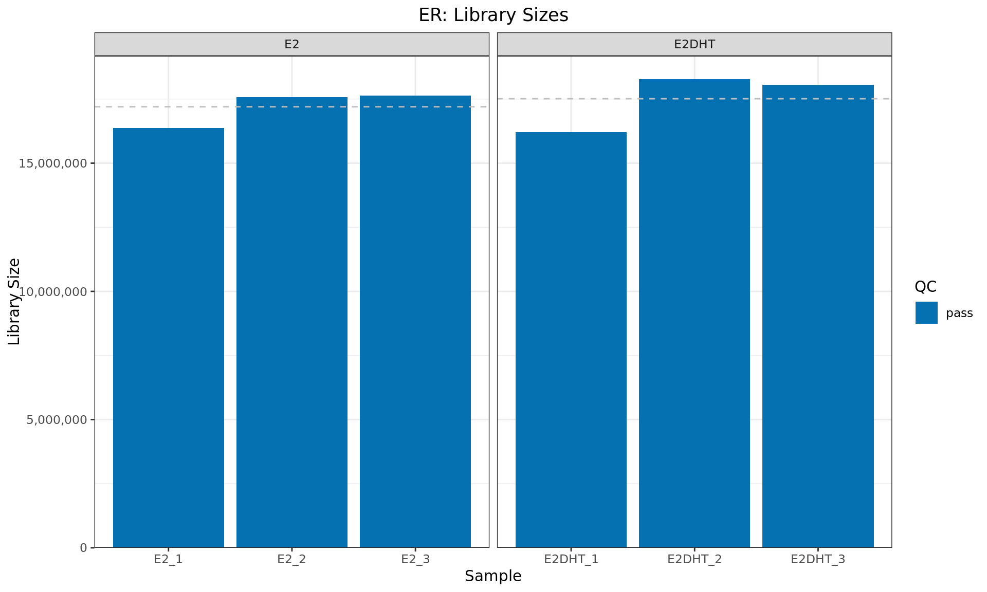
Library sizes for each ER sample. The horizontal line indicates the mean library size for each treatment group. Any samples marked for exclusion as described above will be indicated with an (F)

Peaks Detected

suppressWarnings(
  macs2_logs %>%
    ggplot(aes(label, total_peaks, fill = qc)) +
    geom_col() +
    geom_label(
      aes(x = label, y = total_peaks, label = lab, colour = qc),
      data = . %>%
        dplyr::filter(total_peaks > 0) %>% 
        mutate(
          lab = comma(total_peaks, accuracy = 1), total = total_peaks
        ),
      nudge_y = 0.03 * max(macs2_logs$total_peaks),
      inherit.aes = FALSE, show.legend = FALSE
    ) +
    facet_grid(~treat, scales = "free_x", space = "free_x") +
    scale_y_continuous(expand = expansion(c(0, 0.05)), labels = comma) +
    scale_fill_manual(values = colours$qc) +
    scale_colour_manual(values = colours$qc) +
    labs(
      x = "Sample", y = "Total Peaks", fill = "QC"
    ) +
    ggtitle(glue("{target}: Number of Peaks"))
)

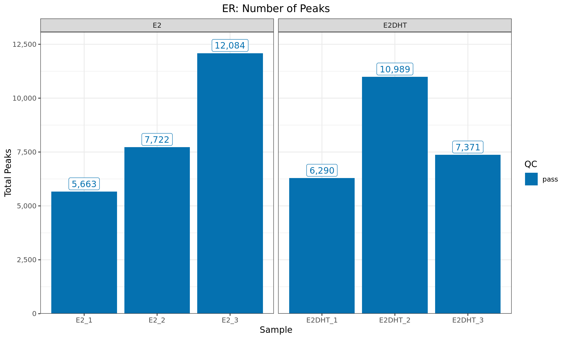
Peaks identified for each ER sample. The number of peaks passing the inclusion criteria for macs2 callpeak (FDR < 0.05) are provided. Any samples marked for exclusion are coloured as indicated in the figure legend.

FRIP

samples$sample %>%
  bplapply(
    function(x) {
      gr <- individual_peaks[[x]]
      rip <- 0
      if (length(gr) > 0) {
        sbp <- ScanBamParam(which = gr)
        rip <- sum(countBam(bfl[[x]], param = sbp)$records)
      }
      tibble(name = x, reads_in_peaks = rip)
    }
  ) %>%
  bind_rows() %>%
  left_join(macs2_logs, by = "name") %>%
  mutate(frip = reads_in_peaks / n_tags_treatment) %>%
  ggplot(aes(label, frip, fill = qc)) +
  geom_col() +
  geom_hline(yintercept = 0.01, colour = "grey", linetype = 2) +
  facet_grid(~treat, scales = "free_x", space = "free") +
  scale_y_continuous(labels = percent, expand = expansion(c(0, 0.05))) +
  scale_fill_manual(values = colours$qc) +
  labs(
    x = "Sample", y = "Fraction of Reads In Peaks", fill = "QC"
  ) +
  ggtitle(glue("{target}: Fraction Of Reads In Peaks"))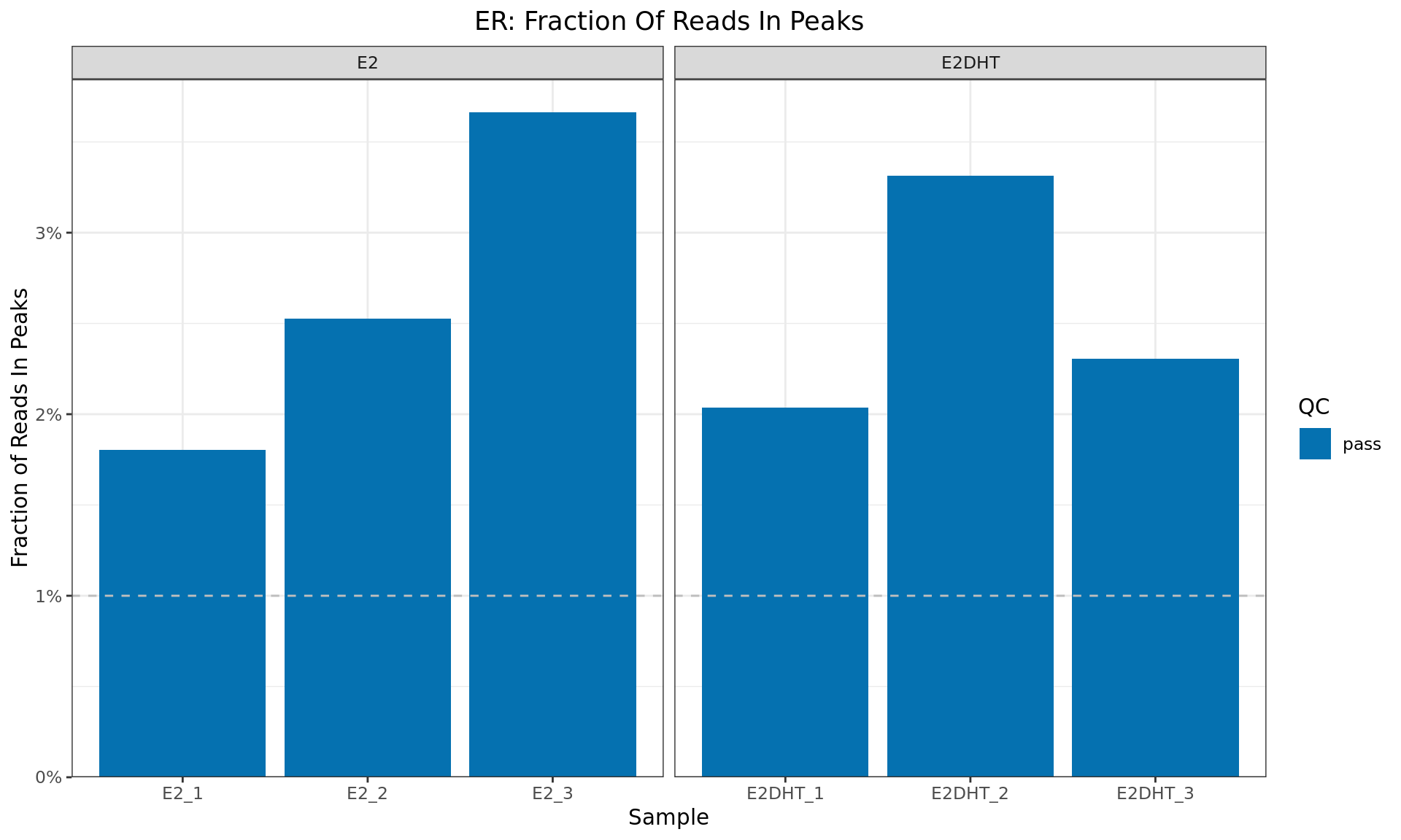

Fraction of Reads In Peaks for each sample. Higher values indicate more reads specifically associated with the ChIP target (ER). The common-use minimum value for an acceptable sample (1%) is shown as a dashed horizontal line

Cross Correlations

macs2_path %>%
  file.path(target, glue("{target}_cross_correlations.tsv")) %>% 
  read_tsv() %>% 
  left_join(samples, by = "sample") %>% 
  ggplot(aes(fl, correlation, colour = treat)) +
  geom_point(alpha = 0.1) +
  geom_smooth(se = FALSE, method = 'gam', formula = y ~ s(x, bs = "cs")) +
  geom_vline(
    aes(xintercept = fragment_length),
    data = macs2_logs,
    colour = "grey40", linetype = 2
  ) +
  geom_label(
    aes(label = fl),
    data = . %>% 
      mutate(correlation = correlation + 0.03 * max(correlation)) %>% 
      dplyr::filter(correlation == max(correlation), .by = sample),
    show.legend = FALSE, alpha = 0.7
  ) +
  facet_grid(as.formula(paste("treat ~", rep_col))) +
  scale_colour_manual(values = colours$treat[treat_levels]) +
  scale_x_continuous(
    breaks = seq(0, 5*max(macs2_logs$fragment_length), by = 200)
  ) +
  labs(
    x = "Distance (bp)", y = "Cross Correlation", colour = "Treat"
  ) +
  ggtitle(glue("{target}: Cross Correlations"))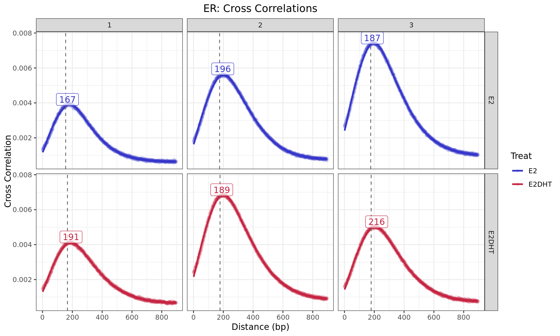

Cross Correlaton between alignments up to 1kb apart. The dashed, grey, vertical line is the fragment length estimated by macs2 callpeak for each sample, with labels indicating the approximate point of the highest correlation, as representative of the average fragment length. For speed, only the first 5 chromosomes were used for sample-specific estimates.

GC Content

ys <- 5e5
yieldSize(bfl) <- ys

bfl %>% 
  bplapply(
    function(x){
      seq <- scanBam(x, param = ScanBamParam(what = "seq"))[[1]]$seq
      freq <- letterFrequency(seq, letters = "GC") / width(seq)
      list(freq[,1])
    }
  ) %>% 
  as_tibble() %>% 
  pivot_longer(
    cols = everything(), 
    names_to = "name",
    values_to = "freq"
  ) %>% 
  left_join(macs2_logs, by = "name") %>% 
  unnest(freq) %>% 
  ggplot(aes(label, freq, fill = qc)) +
  geom_boxplot(alpha = 0.8) +
  geom_hline(
    aes(yintercept = med),
    data = . %>% 
      group_by(treat) %>% 
      summarise(med = median(freq)),
    linetype = 2,
    colour = rgb(0.2, 0.2, 0.8)
  ) +
  facet_grid(~treat, scales = "free_x", space = "free_x") +
  scale_y_continuous(labels = percent) +
  scale_fill_manual(values = colours$qc) +
  labs(
    x = "Sample",
    y = "GC content",
    fill = "QC"
  ) +
  ggtitle(
    glue("{target}: GC Content")
  )

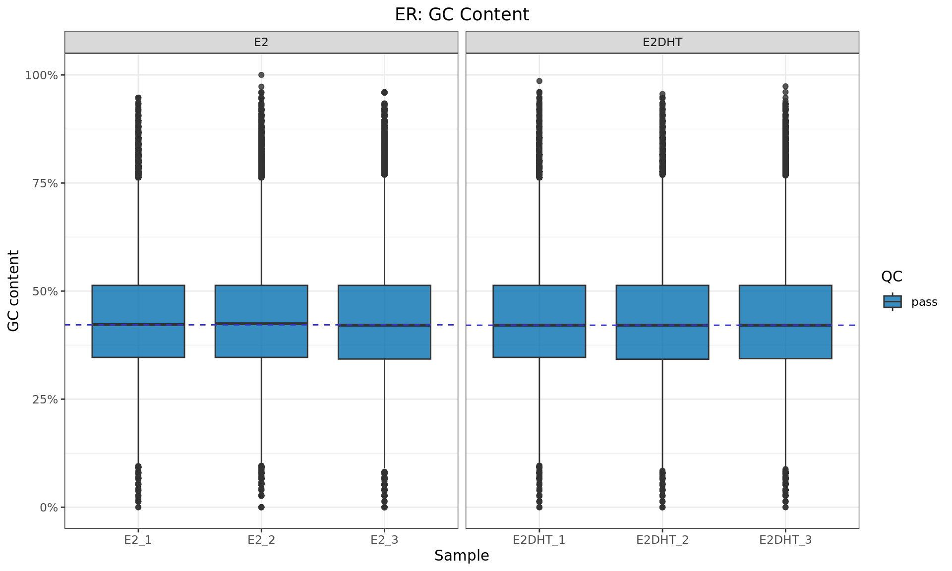
GC content for each bam file, taking the first 500,000 alignments from each sample. QC status is based on the number of peaks identified (see table above)

Results

Individual Replicates

Replicates within treatment groups are only shown where at least one peak was detected. For two or three replicates, Euler (Venn) Diagrams were generated using the python package matplotlib-venn. Peak numbers may differ from above as those shown below are overlapping peaks which have been merged across replicates

In the case of four or more replicates, the package ComplexUpset was used to create UpSet plots (Lex et al. 2014), with colours indicating QC status.

All Samples

sample2label <- setNames(samples$label, samples$sample)
sets <- list(all = paste(samples$label, collapse = "; ")) %>% 
  c(
    samples %>% 
      split(.$treat) %>% 
      lapply(function(x) paste(x$label, collapse = "; "))
  ) %>% 
  unlist()
valid_sets <- makeConsensus(individual_peaks) %>% 
  as_tibble() %>% 
  pivot_longer(
    cols = all_of(samples$sample), names_to = "sample", values_to = "has_peak"
  ) %>% 
  dplyr::filter(has_peak) %>% 
  mutate(sample = sample2label[sample]) %>% 
  summarise(
    samples = paste(sample, collapse = "; "), .by = range
  ) %>% 
  distinct(samples) %>% 
  dplyr::filter(samples %in% sets) %>% 
  pull(samples) %>% 
  setNames(vapply(., function(x){names(which(sets == x))}, character(1))) %>% 
  lapply(function(x) str_split(x, "; ")[[1]])
## Use upset_query objects to fill key intersections and sets
ql <- samples$label %>% 
  lapply(
    function(x) upset_query(
      set = x, 
      fill = colours$treat[as.character(dplyr::filter(samples, label == x)$treat)]
    )
  )
if (length(valid_sets) > 0) {
  ql <- c(
    ql,
    names(valid_sets) %>% 
      lapply(
        function(x) {
          col <- ifelse(x == "all", "darkorange", colours$treat[[x]])
          upset_query(
            intersect = valid_sets[[x]], 
            only_components = "intersections_matrix", 
            color = col, fill = col
          )
        }
      )
  )
}
lb <- rev(arrange(samples, treat)$label)
size <- get_size_mode('exclusive_intersection')
individual_peaks %>% 
  setNames(sample2label[names(.)]) %>% 
  .[lb] %>% 
  plotOverlaps(
    var = "qValue", f = "median",
    .sort_sets = FALSE, queries = ql,
    base_annotations = list(
      `Peaks in Intersection` = intersection_size(
        text_mapping = aes(label = comma(!!size)),
        bar_number_threshold = 1, text_colors = "black", 
        text = list(size = 3.5, angle = 90, vjust = 0.5, hjust = -0.1)
      ) +
        scale_y_continuous(expand = expansion(c(0, 0.25)), label = comma) +
        theme(
          panel.grid = element_blank(), 
          axis.line = element_line(colour = "grey20"),
          panel.border = element_rect(colour = "grey20", fill =  NA)
        )
    ),
    annotations = list(
      qValue = ggplot(mapping = aes(y = qValue)) +
        geom_boxplot(na.rm = TRUE, outlier.colour = rgb(0, 0, 0, 0.2)) +
        coord_cartesian(
          ylim = c(0, quantile(unlist(individual_peaks)$qValue, 0.99))
        ) +
        scale_y_continuous(expand = expansion(c(0, 0.05))) +
        ylab(expr(paste("Macs2 ", q[med]))) +
        theme(
          panel.grid = element_blank(), 
          axis.line = element_line(colour = "grey20"),
          panel.border = element_rect(colour = "grey20", fill =  NA)
        )
    ),
    set_sizes = (
      upset_set_size() +
        geom_text(
          aes(label = comma(after_stat(count))), 
          hjust = 1.1, stat = 'count', size = 3.5
        ) +
        scale_y_reverse(expand = expansion(c(0.3, 0)), label = comma) +
        ylab(glue("Macs2 Peaks (FDR < {config$peaks$macs2$fdr})")) +
        theme(
          panel.grid = element_blank(), 
          axis.line = element_line(colour = "grey20"),
          panel.border = element_rect(colour = "grey20", fill =  NA)
        )
    ),
    min_size = 10, n_intersections = 40
  ) +
  theme(
    panel.grid = element_blank(), 
    panel.border = element_rect(colour = "grey20", fill =  NA),
    axis.line = element_line(colour = "grey20")
  ) +
  labs(x = "Intersection") +
  patchwork::plot_layout(heights = c(2, 3, 2))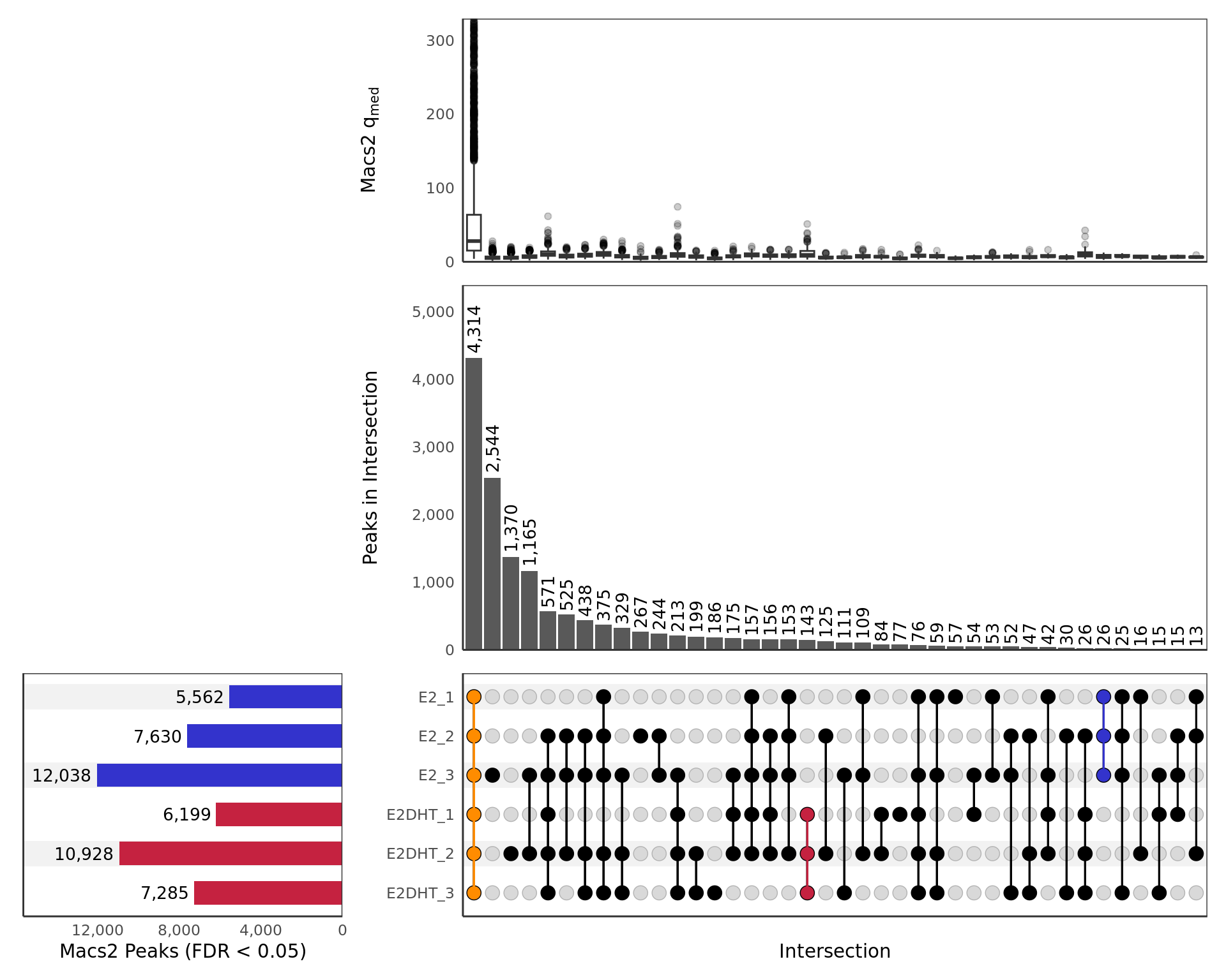

UpSet plot showing all samples including those which failed prior QC steps. Any potential sample mislabelling will show up clearly here as samples from each group should show a preference to overlap other samples within the same treatment group. Intersections are only included if 10 or more sites are present. The top panel shows a boxplot of the median \(q\)-values produced by macs2 callpeak for each peak in the intersection. The y-axis for this panel is truncated at the 99^th percentile of values. Only intersections with 10 or more peaks are shown.

ranges_by_rep_treat <- individual_peaks %>%
  unlist() %>% 
  splitAsList(.$treat) %>% 
  .[vapply(., length, integer(1)) > 1] %>% 
  lapply(select, sample) %>% 
  lapply(reduceMC) %>% 
  lapply(as_tibble) %>% 
  lapply(unnest, sample) %>% 
  lapply(mutate, detected = 1) %>% 
  lapply(left_join, dplyr::select(samples, sample, label), by = "sample") %>%
  lapply(dplyr::select, -sample) %>% 
  lapply(function(x) {
    split(x, x$label) %>% 
      lapply(pull, "range")
    }
  )
## First find the python executable
which_py <- c(
  file.path(Sys.getenv("CONDA_PREFIX"), "bin", "python3"),
  Sys.which("python3")
) %>% 
  .[file.exists(.)] %>% 
  .[1]
stopifnot(length(which_py) == 1)
rep_col <- hcl.colors(3, palette = "Zissou", rev = TRUE)
htmltools::tagList(
  names(ranges_by_rep_treat) %>% 
    lapply(
      function(i) {
        x <- ranges_by_rep_treat[[i]]
        fig_out <- file.path(fig_path, glue("{i}_replicates.{fig_type}"))
        if (length(x) == 1) {
          fig_fun(
            fig_out, 
            width = knitr::opts_chunk$get("fig.width"),
            height = ifelse(
              length(x) < 3,
              knitr::opts_chunk$get("fig.height") * 0.8,
              knitr::opts_chunk$get("fig.height") * 0.8
            )
          )
          grid.newpage()
          draw.single.venn(length(x[[1]]), category = names(x))
          dev.off()
        }
        ## Euler diagrams for 2-3 replicates.
        if (length(x) == 2) {
          a12 <- sum(duplicated(unlist(x)))
          a1 <- length(x[[1]]) - a12 
          a2 <- length(x[[2]]) - a12
          args <- glue(
            here::here("workflow", "scripts", "plot_venn.py "),
            "-a1 {a1} -a2 {a2} -a12 {a12} ",
            "-s1 '{names(x)[[1]]}' -s2 '{names(x)[[2]]}' ", 
            "-c1 '{rep_col[[1]]}' -c2 '{rep_col[[3]]}' ",
            "-ht {knitr::opts_chunk$get('fig.height')} ", 
            "-w {knitr::opts_chunk$get('fig.width')} ", 
            "-o '{fig_out}'"
          )
          system2(which_py, args)
        }
        if (length(x) == 3) {
          a123 <- sum(table(unlist(x)) == 3)
          a12 <- sum(table(unlist(x[1:2])) == 2) - a123
          a13 <- sum(table(unlist(x[c(1, 3)])) == 2) - a123
          a23 <- sum(table(unlist(x[c(2, 3)])) == 2) - a123
          a1 <- length(x[[1]]) - (a12 + a13 + a123)
          a2 <- length(x[[2]]) - (a12 + a23 + a123)
          a3 <- length(x[[3]]) - (a13 + a23 + a123)
          args <- glue(
            here::here("workflow", "scripts", "plot_venn.py "),
            "-a1 {a1} -a2 {a2} -a12 {a12} -a3 {a3} ",
            "-a13 {a13} -a23 {a23} -a123 {a123} ",
            "-s1 '{names(x)[[1]]}' -s2 '{names(x)[[2]]}' -s3 '{names(x)[[3]]}' ", 
            "-c1 '{rep_col[[1]]}' -c2 '{rep_col[[2]]}' -c3 '{rep_col[[3]]}' ",
            "-ht {knitr::opts_chunk$get('fig.height')} ", 
            "-w {knitr::opts_chunk$get('fig.width')} ", 
            "-o '{fig_out}'"
          )
          system2(which_py, args)
        }
        ## An UpSet plot for > 3 replicates
        if (length(x) > 3) {
          fig_fun(
            fig_out, 
            width = knitr::opts_chunk$get("fig.width"),
            height = knitr::opts_chunk$get("fig.height")
          )
          grid.newpage()
          ## Prep the data for ComplexUpset
          df <- individual_peaks[dplyr::filter(samples, treat == i)$sample] %>% 
            makeConsensus(var = "qValue") %>% 
            mutate(qValue = vapply(qValue, median, numeric(1))) %>% 
            as_tibble() %>% 
            dplyr::rename_with(
              function(x) setNames(samples$label, samples$sample)[x],
              any_of(samples$sample)
            )
          ## Highlight samples by QC
          ql <- samples %>% 
            dplyr::filter(treat == i) %>% 
            pull('label') %>% 
            lapply(
              function(x) {
                i <- as.character(
                  dplyr::filter(samples, treat == i, label == x)$qc
                )
                upset_query(set = x, fill = colours$qc[i])
              }
            )
          ## And plot
          p <- df %>% 
            upset(
              intersect = rev(dplyr::filter(samples, treat == i)$label),
              base_annotations = list(
                `Peaks in Intersection` = intersection_size(
                  text_mapping = aes(label = comma(!!size)),
                  bar_number_threshold = 1, text_colors = "black", 
                  text = list(size = 4, hjust = 0.5)
                ) +
                  scale_y_continuous(expand = expansion(c(0, 0.2)), label = comma) +
                  theme(
                    text = element_text(size = 14),
                    panel.grid = element_blank(), 
                    axis.line = element_line(colour = "grey20"),
                    panel.border = element_rect(colour = "grey20", fill =  NA)
                  )
              ),
              annotations = list(
                qValue = ggplot(mapping = aes(y = qValue)) +
                  geom_boxplot(na.rm = TRUE, outlier.colour = rgb(0, 0, 0, 0.2)) +
                  coord_cartesian(ylim = c(0, quantile(df$qValue, 0.99))) +
                  scale_y_continuous(expand = expansion(c(0, 0.05))) +
                  ylab(expr(paste("Macs2 ", q[med]))) +
                  theme(
                    text = element_text(size = 14),
                    panel.grid = element_blank(), 
                    axis.line = element_line(colour = "grey20"),
                    panel.border = element_rect(colour = "grey20", fill =  NA)
                  )
              ),
              set_sizes = (
                upset_set_size() +
                  geom_text(
                    aes(label = comma(after_stat(count))), 
                    hjust = 1.1, stat = 'count', size = 4
                  ) +
                  scale_y_reverse(expand = expansion(c(0.2, 0)), label = comma) +
                  ylab(glue("Macs2 Peaks (FDR < {config$peaks$macs2$fdr})")) +
                  theme(
                    text = element_text(size = 14),
                    panel.grid = element_blank(), 
                    axis.line = element_line(colour = "grey20"),
                    panel.border = element_rect(colour = "grey20", fill =  NA)
                  )
              ),
              queries = ql,
              min_size = 10,
              sort_sets = FALSE
            ) +
            theme(text = element_text(size = 14)) +
            patchwork::plot_layout(heights = c(2, 3, 2))
          print(p)
          dev.off()
        }
        
        ## Define the caption
        cp <- htmltools::tags$em(
          glue(
            "
            Number of {target} peaks detected by macs2 callpeak in each {i} 
            replicate and the number of peaks shared between replicates. 
            Replicates which passed/failed QC are show in the specified colours.
            "
          )
        )
        
        ## Create html tags
        fig_link <- str_extract(fig_out, "assets.+")
        htmltools::div(
          htmltools::div(
            id = glue("{i}-replicates"),
            class = "section level4",
            htmltools::h4(i),
            htmltools::div(
              class = "figure", style = "text-align: center",
              htmltools::img(src = fig_link, width = 960),
              htmltools::p(
                class = "caption", htmltools::tags$em(cp)
              )
            )
          )
        )
      }
    )
)

E2

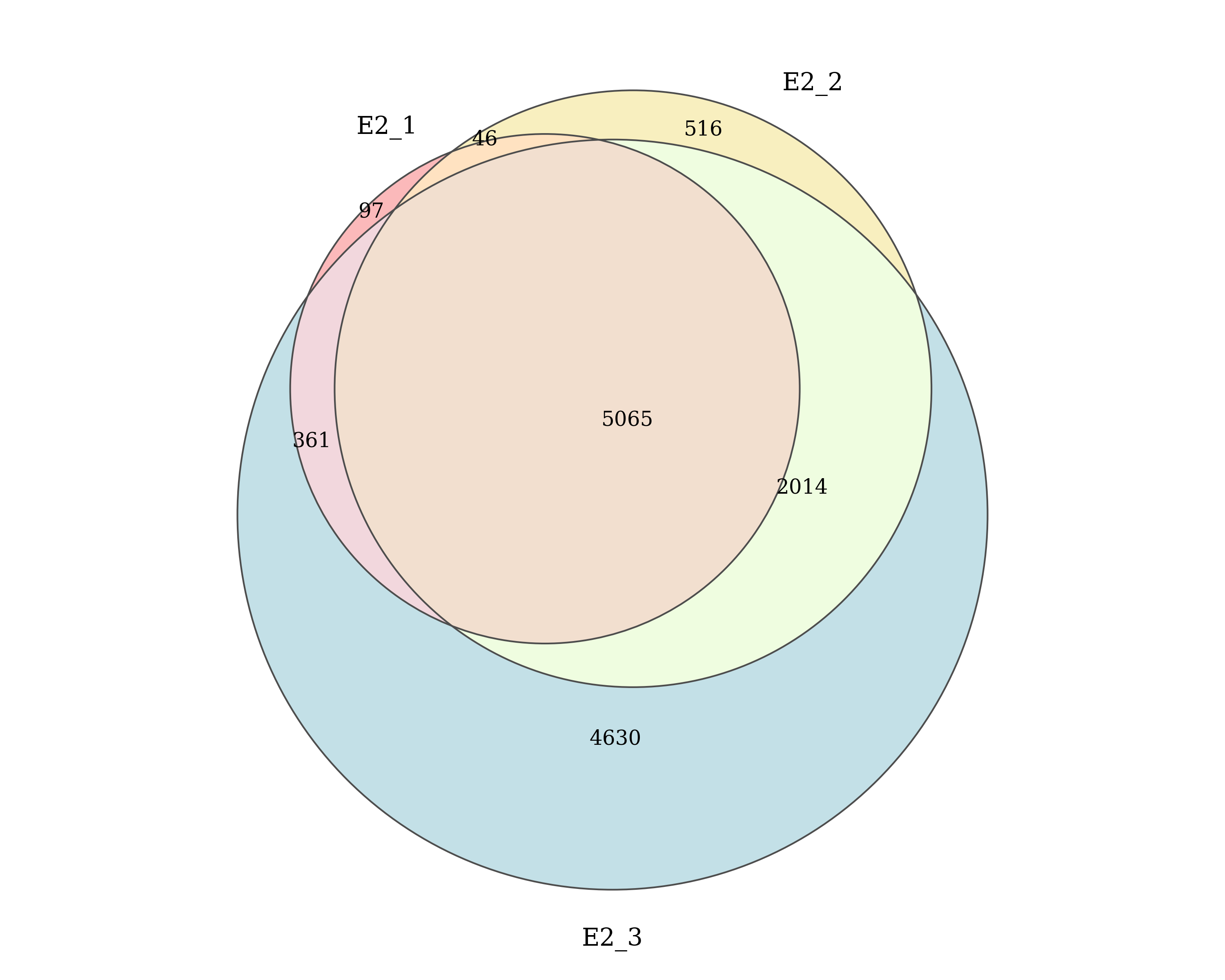
Number of ER peaks detected by macs2 callpeak in each E2 replicate and the number of peaks shared between replicates. Replicates which passed/failed QC are show in the specified colours.

E2DHT

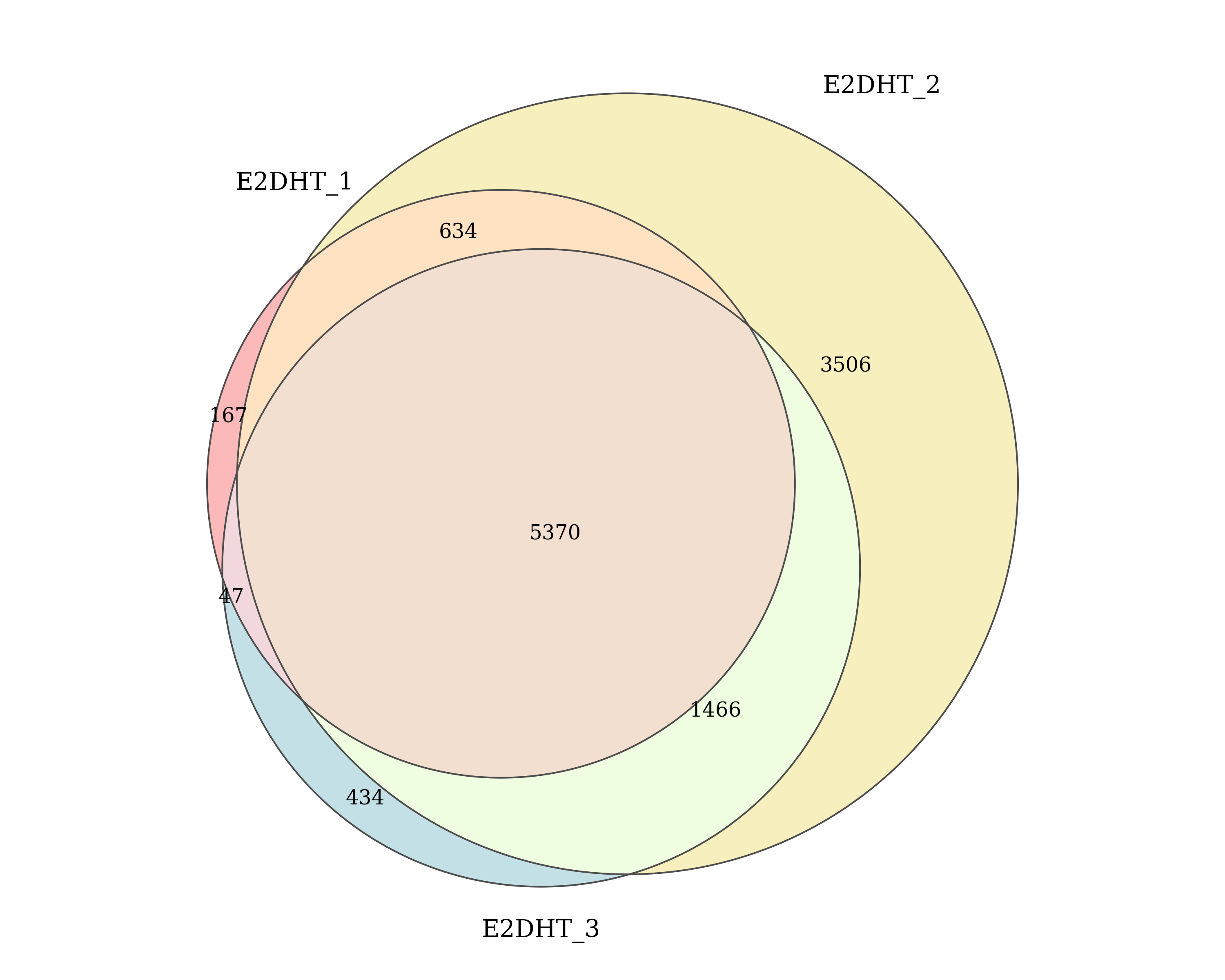
Number of ER peaks detected by macs2 callpeak in each E2DHT replicate and the number of peaks shared between replicates. Replicates which passed/failed QC are show in the specified colours.

Individual Peak Widths

individual_peaks %>% 
  width() %>% 
  as.list() %>% 
  lapply(list) %>% 
  as_tibble() %>% 
  pivot_longer(cols = everything(), names_to = "sample", values_to = "width") %>% 
  unnest(width) %>% 
  left_join(samples, by = "sample") %>% 
  ggplot(aes(label, width, fill = treat)) +
  geom_boxplot(alpha = 0.9) +
  geom_hline(
    yintercept = median(width(unlist(individual_peaks))),
    linetype = 2
  ) +
  facet_wrap(~treat, nrow = 1, scales = "free_x") +
  scale_y_log10() +
  scale_fill_manual(values = colours$treat) +
  labs(x = "Sample", y = "Peak Width (bp)", fill = "Treatment")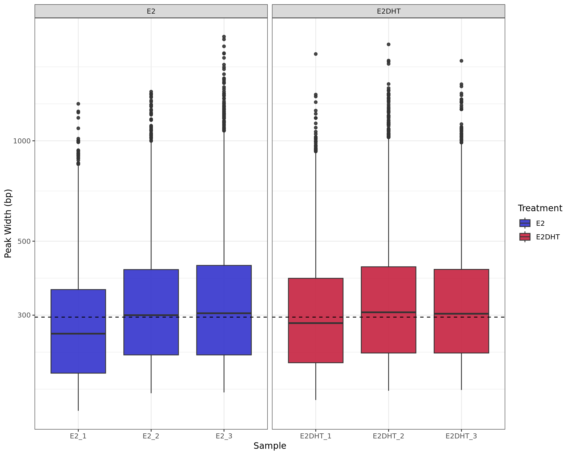

Range of peak widths across all samples. The median value for all peaks (296bp) is shown as the dashed horizontal line

Treatment Peaks

treatment_peaks <- treat_levels %>%
  sapply(
    function(x) {
      gr <- macs2_path %>%
        file.path(target, glue("{target}_{x}_merged_peaks.narrowPeak")) %>%
        importPeaks(seqinfo = sq, blacklist = blacklist, centre = TRUE) %>% 
        unlist()
      k <- dplyr::filter(n_reps, treat == x)$n * config$peaks$qc$min_prop_reps
      if (k > 0) {
        samp <- dplyr::filter(macs2_logs, treat == x, qc != "fail")$name
        gr$n_reps <- countOverlaps(gr, individual_peaks[samp]) 
        gr$keep <- gr$n_reps >= k
      } else {
        gr <- GRanges(seqinfo = sq)
      }
      gr
    },
    simplify = FALSE
  ) %>%
  GRangesList() 
union_peaks <- treatment_peaks %>% 
  endoapply(subset, keep) %>% 
  makeConsensus(
    var = c("score", "signalValue", "pValue", "qValue", "centre")
  ) %>% 
  mutate(
    score = vapply(score, median, numeric(1)),
    signalValue = vapply(signalValue, median, numeric(1)),
    pValue = vapply(pValue, median, numeric(1)),
    qValue = vapply(qValue, median, numeric(1)),
    centre = vapply(centre, median, numeric(1)),
    region = bestOverlap(
      ., 
      lapply(gene_regions, select, region) %>% 
        GRangesList() %>% 
        unlist(),
      var = "region"
    ) %>% 
      factor(levels = regions)
  ) 
if (has_features) {
  union_peaks$Feature <- bestOverlap(
    union_peaks, external_features, 
    var = "feature", missing = "no_feature"
  ) %>% 
    factor(levels = names(colours$features)) %>% 
    fct_relabel(str_sep_to_title)
}

A set of treatment-specific ER peaks (i.e. treatment peaks) was defined for each condition by comparing the peaks detected when merging all treatment-specific samples, against those detected within each replicate. Replicates which failed the previous QC steps are omitted from this step. Treatment peaks which overlapped a peak in more than 50% of the individual replicates passing QC in each treatment group, were retained.

treatment_peaks %>%
  lapply(
    function(x) {
      tibble(
        detected_peaks = length(x),
        retained = sum(x$keep),
        `% retained` = percent(retained / detected_peaks, 0.1),
        median_width = median(width(x))
      )
    }
  ) %>% 
  bind_rows(.id = "treat") %>% 
  mutate(treat = factor(treat, levels = treat_levels)) %>% 
  group_by(treat) %>% 
  rename_all(str_sep_to_title) %>% 
  dplyr::rename(`% Retained` = ` Retained`) %>% 
  pander(
    justify = "lrrrr",
    caption = glue(
      "Treatment peaks detected by merging samples within each treatment group.",
      "Peaks were only retained if detected in at least",
      "{percent(config$peaks$qc$min_prop_reps)} of the retained samples for each", "treatment group, as described above.",
      .sep = " "
    )
  )

Treatment peaks detected by merging samples within each treatment group. Peaks were only retained if detected in at least 50% of the retained samples for each treatment group, as described above.
Treat	Detected Peaks	Retained	% Retained	Median Width
E2	7,335	6,673	91.0%	296
E2DHT	7,129	6,835	95.9%	298

Union Peaks

vd <- treatment_peaks %>%
    lapply(
      function(x) {
        as.character(
          subsetByOverlaps(
            union_peaks, 
            subset(x, keep)
          )
        )
      }
    ) %>%
    setNames(treat_levels) %>%
    .[vapply(., length, integer(1)) > 0]

In addition to the treatment peaks, a set of 7,532 treatment-agnostic ER union peaks were defined. Union ranges were the union of all overlapping ranges defined and retained in one or more sets of treatment peaks. Resulting values for the score, signalValue, pValue and qValue were calculated as the median across all treatments. Peak summits were taken as the median position of all summits which comprise the union peak.

Venn Diagram

fig_name <- glue("{target}_common_peaks.{fig_type}")
fig_out <- file.path(fig_path, fig_name)
## An empty file to keep snakemake happy if > 3 treatments
file.create(fig_out) 
if (length(vd) == 1) {
  fig_fun(filename = fig_out, width = 8, height = 3)
  grid.newpage()
  draw.single.venn(
    area = length(vd[[1]]), category = names(vd)[[1]], 
    fill = colours$treat[names(vd)], alpha = 0.3
  )
  dev.off()
}
if (length(vd) == 2) {
  a1 <- length(setdiff(vd[[1]], vd[[2]]))
  a2 <- length(setdiff(vd[[2]], vd[[1]]))
  a12 <- sum(duplicated(unlist(vd)))
  args <- glue(
    here::here("workflow", "scripts", "plot_venn.py "),
    "-a1 {a1} -a2 {a2} -a12 {a12} ",
    "-s1 '{names(vd)[[1]]}' -s2 '{names(vd)[[2]]}' ", 
    "-c1 '{colours$treat[[names(vd)[[1]]]]}' ",
    "-c2 '{colours$treat[[names(vd)[[2]]]]}' ",
    "-ht {knitr::opts_chunk$get('fig.height')} ", 
    "-w {knitr::opts_chunk$get('fig.width')} ", 
    "-o '{fig_out}'"
  )
  system2(which_py, args)
}
if (length(vd) == 3) {
  a123 <- sum(table(unlist(vd)) == 3)
  a12 <- sum(table(unlist(vd[1:2])) == 2) - a123
  a13 <- sum(table(unlist(vd[c(1, 3)])) == 2) - a123
  a23 <- sum(table(unlist(vd[c(2, 3)])) == 2) - a123
  a1 <- length(vd[[1]]) - (a12 + a13 + a123)
  a2 <- length(vd[[2]]) - (a12 + a23 + a123)
  a3 <- length(vd[[3]]) - (a13 + a23 + a123)
  args <- glue(
    here::here("workflow", "scripts", "plot_venn.py "),
    "-a1 {a1} -a2 {a2} -a12 {a12} -a3 {a3} ",
    "-a13 {a13} -a23 {a23} -a123 {a123} ",
    "-s1 '{names(vd)[[1]]}' -s2 '{names(vd)[[2]]}' -s3 '{names(vd)[[3]]}' ", 
    "-c1 '{colours$treat[[names(vd)[[1]]]]}' ",
    "-c2 '{colours$treat[[names(vd)[[2]]]]}' ",
    "-c3 '{colours$treat[[names(vd)[[3]]]]}' ",
    "-ht {knitr::opts_chunk$get('fig.height')} ", 
    "-w {knitr::opts_chunk$get('fig.width')} ", 
    "-o '{fig_out}'"
  )
  system2(which_py, args)
}

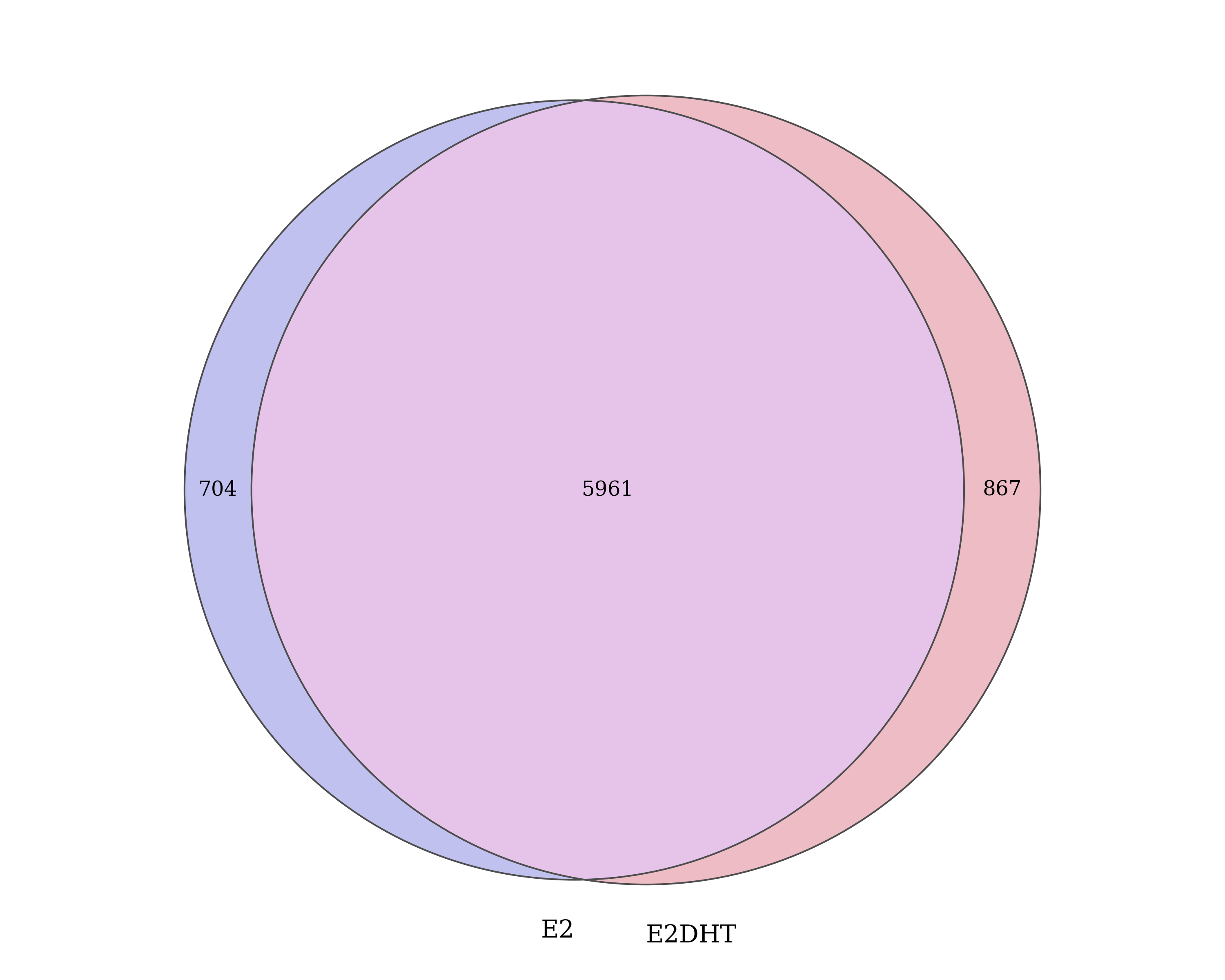
Number of ER union peaks which overlap treatment peaks defined within each condition.

Distance to TSS

a <- union_peaks %>% 
  join_nearest(
    mutate(tss, tss = start)
  ) %>% 
  mutate(d = start + width/2 - tss) %>% 
  as_tibble() %>% 
  ggplot(aes(d / 1e3)) +
  geom_density() +
  coord_cartesian(xlim = c(-100, 100)) +
  labs(
    x = "Distance to Nearest TSS (kb)",
    y = "Density"
  )
b <- union_peaks %>% 
  join_nearest(
    mutate(tss, tss = start)
  ) %>% 
  mutate(d = start + width/2 - tss) %>%
  as_tibble() %>% 
  select(d) %>% 
  arrange(abs(d)) %>% 
  mutate(
    q = seq_along(d) / nrow(.)
  ) %>% 
  ggplot(aes(abs(d) / 1e3, q)) +
  geom_line() +
  geom_vline(
    xintercept = max(unlist(extra_params$gene_regions$promoters)) / 1e3, 
    linetype = 2, colour = "grey40"
  ) +
  coord_cartesian(xlim = c(0, 100)) +
  labs(
    x = "Distance to Nearest TSS (kb)",
    y = "Percentile"
  ) +
  scale_y_continuous(labels = percent, breaks = seq(0, 1, by = 0.2)) +
  scale_x_continuous(breaks = seq(0, 100, by = 20))
a + b + plot_annotation(tag_levels = "A")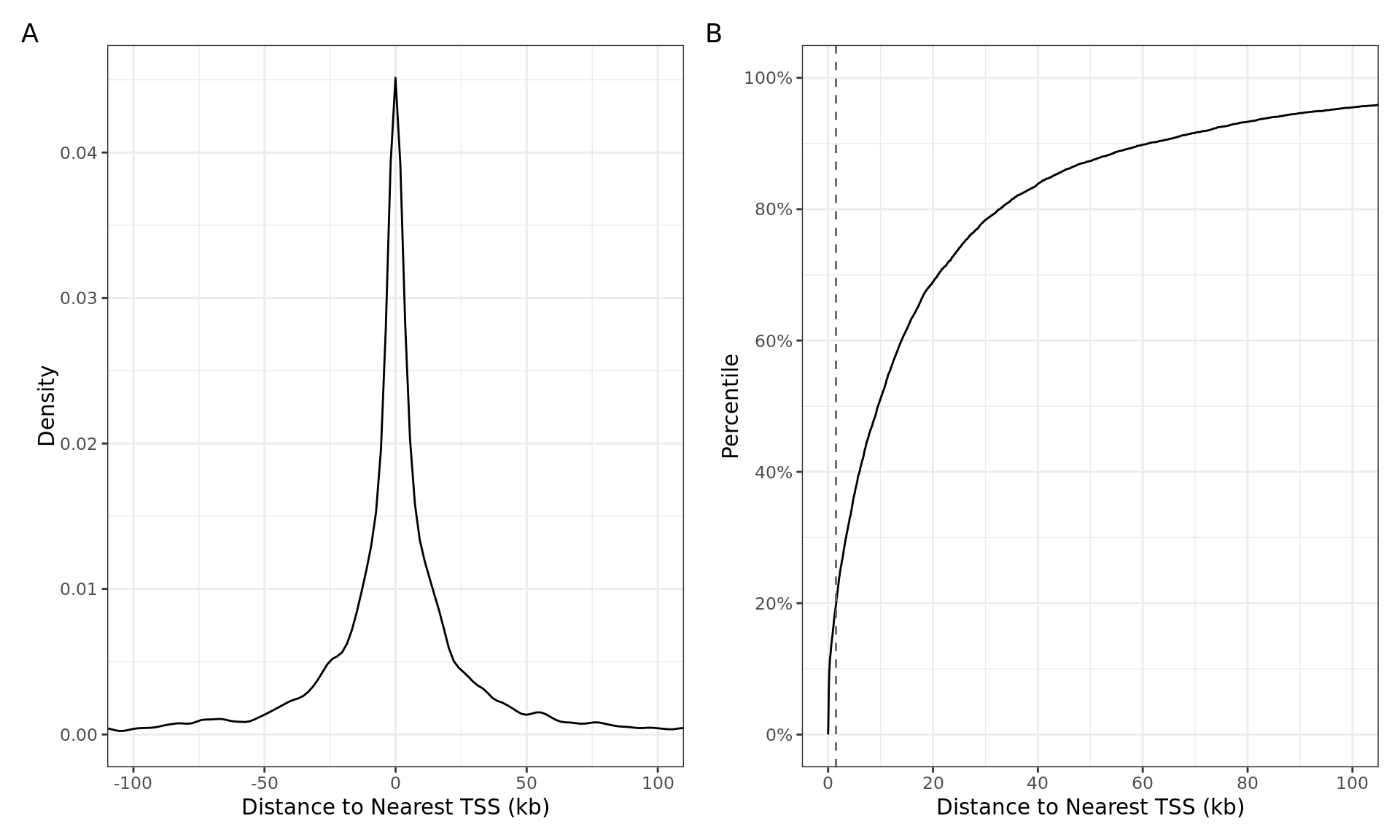

Distances from the centre of the ER union peak to the transcription start-site shown as A) a histogram, and B) as a cumulative distribution. The vertical dashed line indicates the range considered to be a promoter during annotation preparation. 637 of the 7,532 ER union peaks (8.5%) directly overlapped a TSS.

Gene-Centric Regions

union_peaks %>% 
  plotPie(
    fill = "region", total_size = 4,
    cat_glue = "{str_wrap(.data[[fill]], 15)}\n{comma(n, 1)}\n({percent(p, 0.1)})",
    cat_alpha = 0.9, cat_adj = 0.05, min_p = 0.025
  ) +
  scale_fill_manual(
    values = colours$regions %>% setNames(regions[names(.)])
  ) +
  theme(legend.position = "none")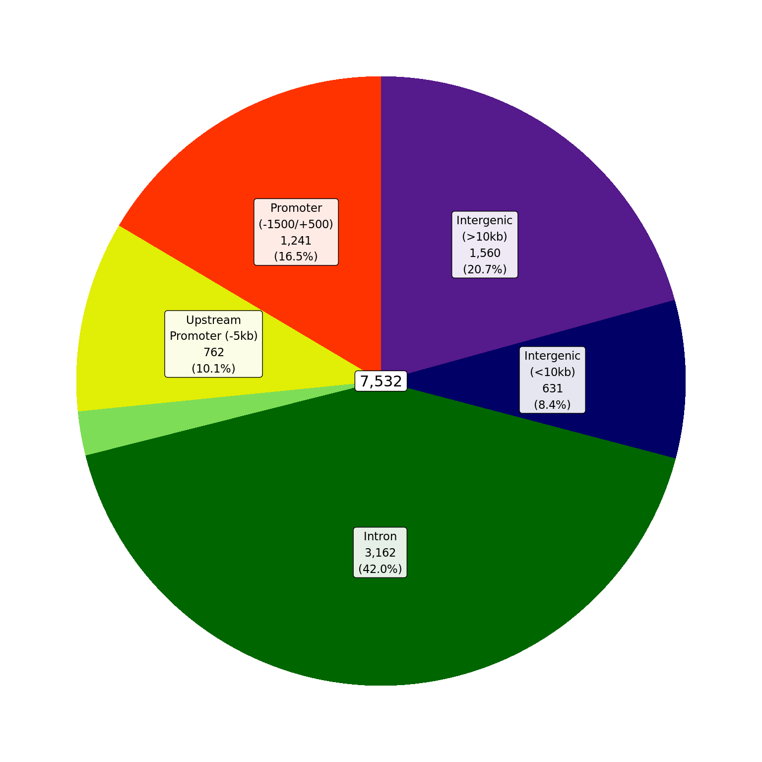

Proportions of ER union peaks which overlap gene-centric features.

External Features

union_peaks %>% 
  plotPie(
    fill = "Feature", total_size = 4,
    cat_glue = "{str_wrap(.data[[fill]], 15)}\n{comma(n, 1)}\n({percent(p, 0.1)})",
    cat_alpha = 0.9, cat_adj = 0.05
  ) +
  scale_fill_manual(
    values = colours$features %>% setNames(str_sep_to_title(names(.)))
  ) +
  theme(legend.position = "none")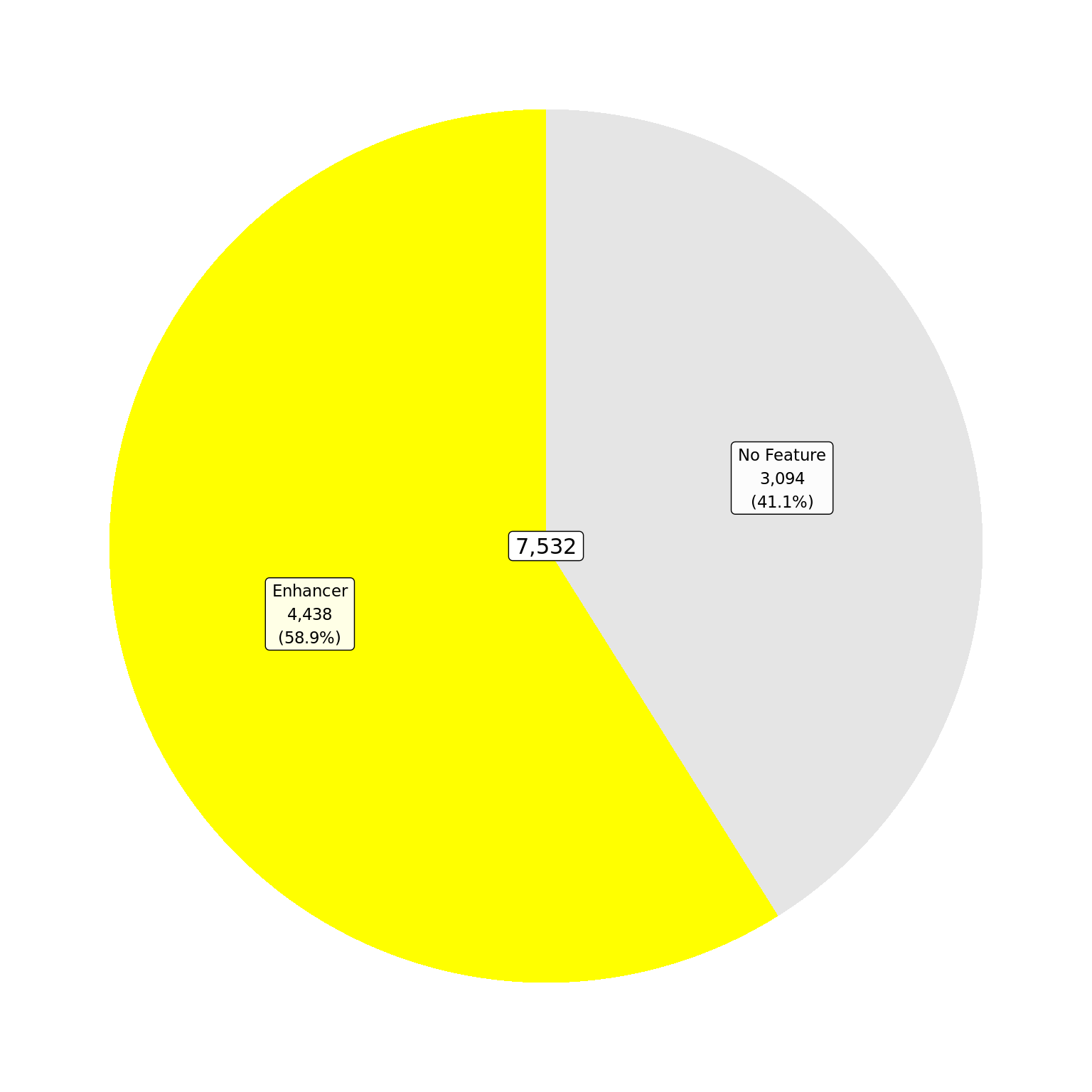

The total number of ER union peaks which overlap external features provided in enhancer_atlas_2.0_zr75.gtf.gz. If peaks map to multiple features, they are assigned to the one with the largest overlap.

External Features And Gene-Centric Regions

union_peaks %>% 
  plotSplitDonut(
    inner = "Feature", outer = "region",
    inner_palette = colours$features %>% setNames(str_to_title(names(.))),
    outer_palette = colours$regions %>% setNames(regions[names(.)]),
    inner_glue = "{str_wrap(.data[[inner]], 15)}\nn = {comma(n, 1)}\n{percent(p,0.1)}",
    outer_glue = "{str_wrap(.data[[outer]], 15)}\nn = {comma(n, 1)}\n{percent(p,0.1)}",
    min_p = 0.03, outer_alpha = 0.8
  )

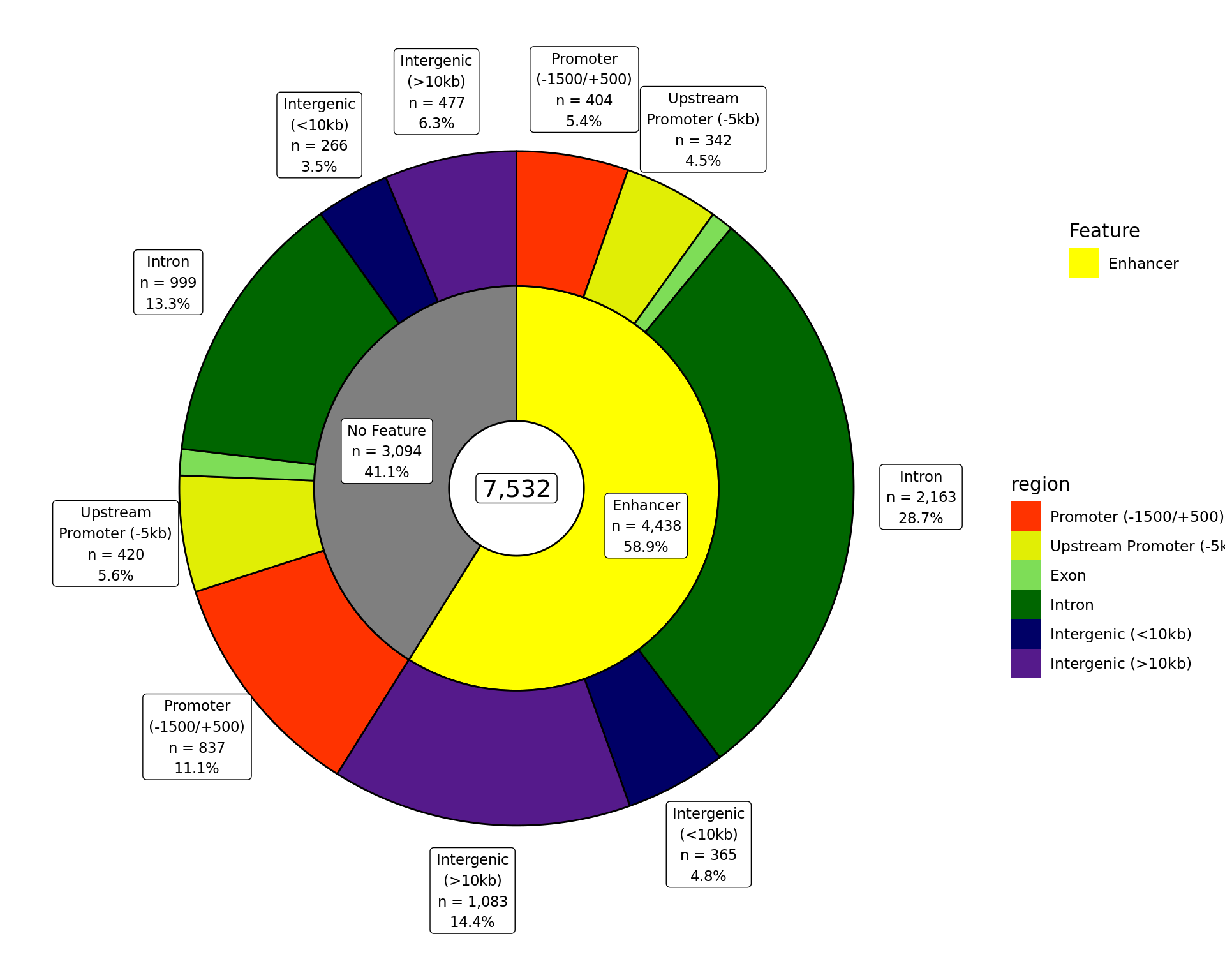
The total number of ER union peaks overlapping external features and gene-centric regions. If a peak overlaps multiple features or regions, it is assigned to be the one with the largest overlap. Any peaks which don’t overlap a feature have been excluded.

Highly Ranked Peaks

grl_to_plot <- vector("list", length(treat_levels) + 1) %>%
  setNames(c("union", treat_levels))
grl_to_plot$union <- union_peaks %>%
  as_tibble() %>%
  arrange(desc(score)) %>%
  dplyr::slice(1) %>%
  colToRanges("range", seqinfo = sq)
grl_to_plot[treat_levels] <- treat_levels %>% 
  lapply(
    function(x) {
      if (length(treatment_peaks[[x]]) == 0) return(NULL)
      tbl <- treatment_peaks[[x]] %>% 
        filter(keep) %>% 
        filter_by_non_overlaps(
          unlist(treatment_peaks[setdiff(treat_levels, x)])
        ) %>% 
        filter_by_non_overlaps(grl_to_plot$union) %>% 
        as_tibble() 
      if (nrow(tbl) == 0) return(NULL)
      tbl %>% 
        arrange(desc(score)) %>% 
        dplyr::slice(1) %>% 
        colToRanges("range", seqinfo = sq)
    }
  )
grl_to_plot <- grl_to_plot %>% 
  .[vapply(., length, integer(1)) > 0] %>% 
  lapply(setNames, NULL) %>% 
  GRangesList() %>% 
  unlist() %>% 
  distinctMC(.keep_all = TRUE) %>% 
  splitAsList(names(.)) %>% 
  endoapply(function(x) x[1,]) %>% 
  .[intersect(c("union", treat_levels), names(.))]

## The coverage
bwfl <- list2(
  "{target}" := macs2_path %>%
  file.path(target, glue("{target}_{treat_levels}_merged_treat_pileup.bw")) %>% 
  BigWigFileList() %>% 
  setNames(treat_levels)
)
## The features track
feat_gr <- gene_regions %>% 
  lapply(granges) %>% 
  GRangesList()
feature_colours <- colours$regions
if (has_features) {
  feat_gr <- list(Regions = feat_gr)
  feat_gr$Features <- splitAsList(external_features, external_features$feature)
  feature_colours <- list(
    Regions = unlist(colours$regions),
    Features = unlist(colours$features)
  )
}
## The genes track defaults to transcript models
hfgc_genes <- read_rds(
  here::here("output", "annotations", "trans_models.rds")
)
gene_col <- "grey"
## If RNA-Seq data is present, the genes track switches to Up/Down etc
if (nrow(rnaseq)) {
  rna_lfc_col <- colnames(rnaseq)[str_detect(str_to_lower(colnames(rnaseq)), "logfc")][1]
  rna_fdr_col <- colnames(rnaseq)[str_detect(str_to_lower(colnames(rnaseq)), "fdr|adjp")][1]
  if (!is.na(rna_lfc_col) & !is.na(rna_fdr_col)) {
    hfgc_genes <- hfgc_genes %>%
      mutate(
        status = case_when(
          !gene %in% rnaseq$gene_id ~ "Undetected",
          gene %in% dplyr::filter(
            rnaseq, !!sym(rna_lfc_col) > 0, !!sym(rna_fdr_col) < fdr_alpha
          )$gene_id ~ "Up",
          gene %in% dplyr::filter(
            rnaseq, !!sym(rna_lfc_col) < 0, !!sym(rna_fdr_col) < fdr_alpha
          )$gene_id ~ "Down",
          gene %in% dplyr::filter(
            rnaseq, !!sym(rna_fdr_col) >= fdr_alpha
          )$gene_id ~ "Unchanged"
        )
      ) %>%
      splitAsList(.$status) %>%
      lapply(select, -status) %>%
      GRangesList()
    gene_col <- colours$direction %>%
      setNames(str_to_title(names(.)))
  }
}
## External Coverage (Optional)
if (!is.null(config$external$coverage)) {
  ext_cov_path <- config$external$coverage %>% 
    lapply(unlist) %>% 
    lapply(function(x) setNames(here::here(x), names(x)))
  bwfl <- c(
    bwfl[target],
    config$external$coverage %>% 
      lapply(
        function(x) {
          BigWigFileList(here::here(unlist(x))) %>% 
            setNames(names(x))
        }
      )
  )
}
line_col <- lapply(bwfl, function(x) colours$treat[names(x)])
y_lim <- bwfl %>%
  lapply(
    function(x) {
      gr <- unlist(grl_to_plot) %>% 
        resize(width = 30 * width(.), fix = 'center')
      x %>% 
        lapply(import.bw, which = gr) %>%
        lapply(function(rng) c(0, max(rng$score))) %>%
        unlist() %>%
        range()
    }
  )

Coverage for a small set of highly ranked peaks are shown below. These are the most highly ranked Union Peak (by score) and any treatment peaks which are unique to each treatment group, after excluding the most highly ranked union peak.

htmltools::tagList(
  mclapply(
    seq_along(grl_to_plot),
    function(x) {
      nm <- names(grl_to_plot)[[x]]
      ## Export the figure
      fig_out <- file.path(
        fig_path,
        nm %>% 
          str_replace_all(" ", "_") %>% 
          paste0("_topranked.", fig_type)
      )
      fig_fun(
        filename = fig_out,
        width = knitr::opts_current$get("fig.width"), 
        height = knitr::opts_current$get("fig.height")
      )
      ## Automatically collapse Transcripts if more than 10
      ct <- FALSE
      gh <- 1
      if (length(subsetByOverlaps(gtf_transcript, grl_to_plot[[x]])) > 20) {
        ct <- "meta"
        gh <- 0.5
      }
      ## Generate the plot
      plotHFGC(
        grl_to_plot[[x]],
        features = feat_gr, featcol = feature_colours, featsize = 1 + has_features,
        genes = hfgc_genes, genecol = gene_col,
        coverage = bwfl, linecol = line_col,
        cytobands = bands_df,
        rotation.title = 90,
        zoom = 30,
        ylim = y_lim,
        collapseTranscripts = ct, genesize = gh,
        col.title = "black", background.title = "white", 
        showAxis = FALSE
      )
      dev.off()
      
      ## Define the caption
      gr <- join_nearest(grl_to_plot[[x]], gtf_gene, distance = TRUE)
      d <- gr$distance
      gn <- gr$gene_name
      peak_desc <- ifelse(
        nm == "union",
        "union peak by combined score across all treatments.",
        paste(
          "treatment-peak unique to the merged", nm, "samples."
        )
      )
      cp <- htmltools::tags$em(
        glue(
          "The most highly ranked {peak_desc} ",
          ifelse(
            d == 0,
            paste('The peak directly overlaps', gn),
            paste0("The nearest gene was ", gn, ", ", round(d/1e3, 1), "kb away")
          ),
          ifelse(
            (nrow(rnaseq) > 0) & (gn %in% gtf_gene$gene_name),
            glue(" which was detected in the RNA-Seq data."),
            glue(".")
          ),
          "
          Y-axes for each coverage track are set to the most highly ranked peak
          across all conditions.
          "
        )
      )
      
      ## Create html tags
      fig_link <- str_extract(fig_out, "assets.+")
      htmltools::div(
        htmltools::div(
          id = nm %>% 
            str_replace_all(" ", "-") %>% 
            str_to_lower() %>% 
            paste0("-topranked"),
          class = "section level3",
          htmltools::h3(
            ifelse(
              nm == "union",
              "Union Peaks",
              paste("Treatment Peaks:", nm)
            )
          ),
          htmltools::div(
            class = "figure", style = "text-align: center",
            htmltools::img(src = fig_link, width = 960),
            htmltools::p(
              class = "caption", htmltools::tags$em(cp)
            )
          )
        )
      )
    },
    mc.cores = min(length(grl_to_plot), threads)
  )
)

Union Peaks

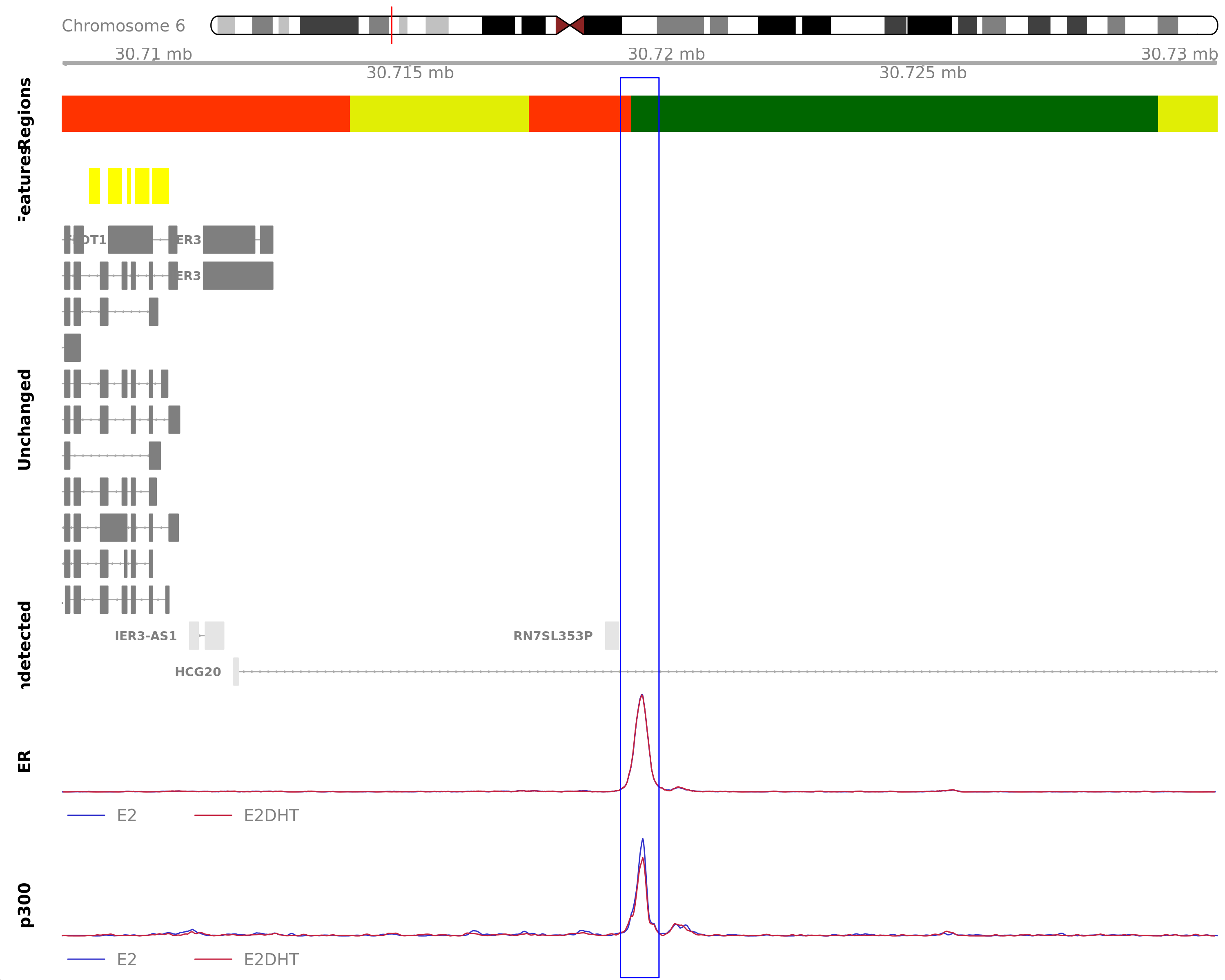
The most highly ranked union peak by combined score across all treatments. The nearest gene was IER3, 6.8kb away which was detected in the RNA-Seq data. Y-axes for each coverage track are set to the most highly ranked peak across all conditions.

Treatment Peaks: E2

The most highly ranked treatment-peak unique to the merged E2 samples. The nearest gene was IRS2, 108.3kb away which was detected in the RNA-Seq data. Y-axes for each coverage track are set to the most highly ranked peak across all conditions.

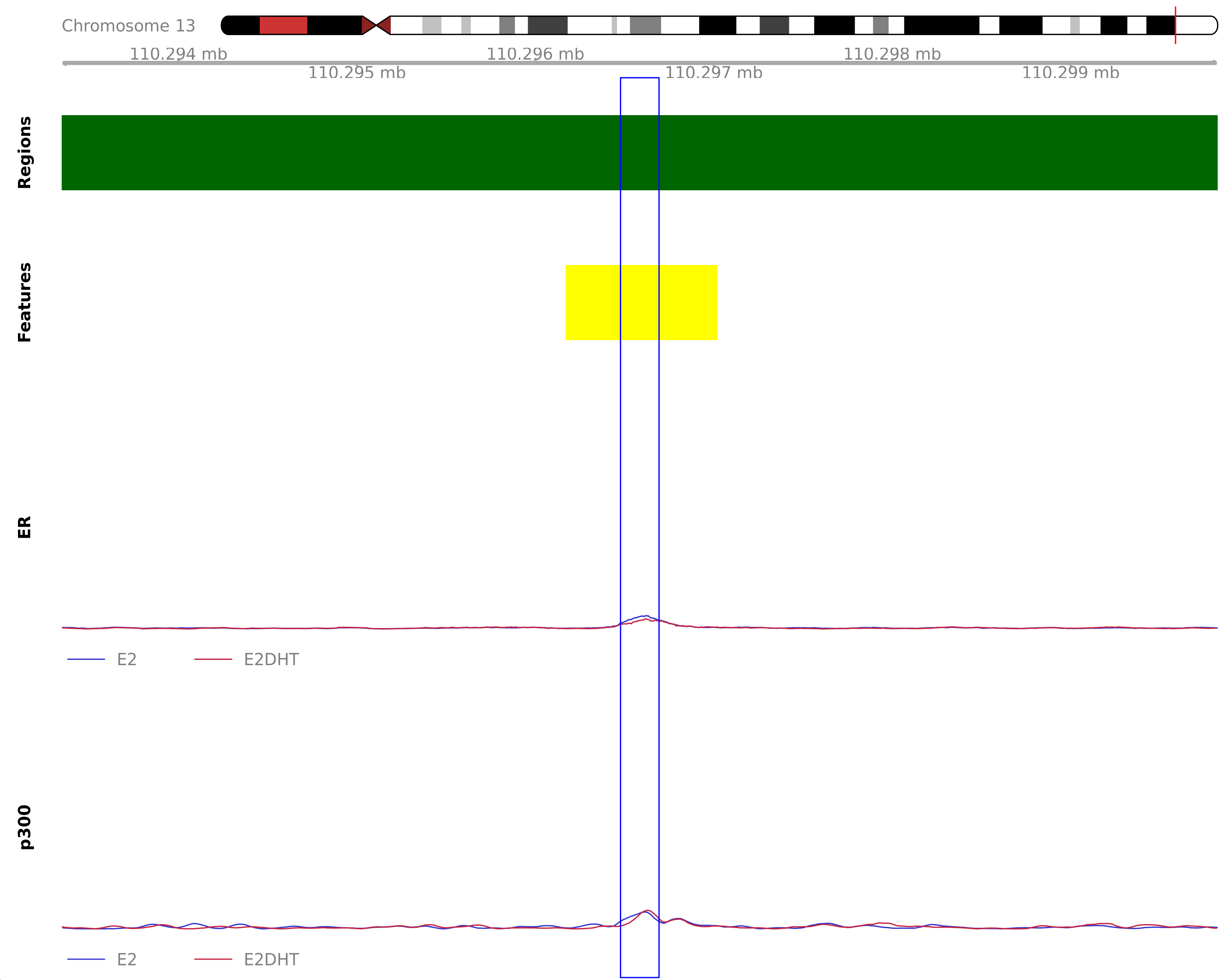
Treatment Peaks: E2DHT

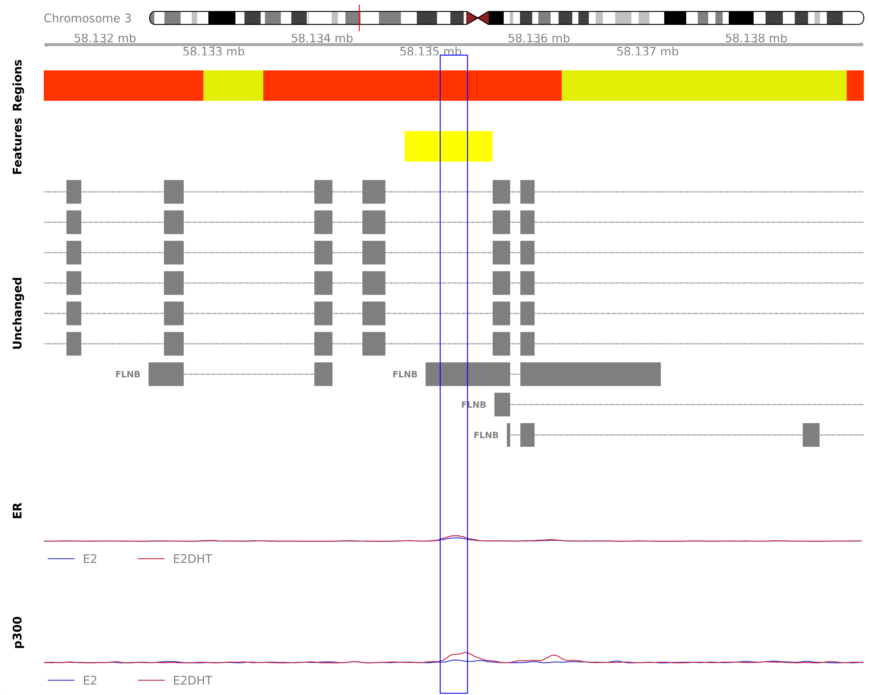
The most highly ranked treatment-peak unique to the merged E2DHT samples. The peak directly overlaps FLNB which was detected in the RNA-Seq data. Y-axes for each coverage track are set to the most highly ranked peak across all conditions.

Data Export

all_out <- list(
  union_peaks_bed = file.path(
    macs2_path, target, glue("{target}_union_peaks.bed")
  ),
  treatment_peaks_rds = file.path(
    macs2_path, target, glue("{target}_treatment_peaks.rds")),
  renv = file.path(
    here::here("output/envs"), glue("{target}_macs2_summary.RData")
  )
) %>% 
  c(
    sapply(
      names(treatment_peaks), 
      function(x) {
        file.path(
          macs2_path, target, glue("{target}_{x}_treatment_peaks.bed")
        )
      },
      simplify = FALSE
    ) %>% 
      setNames(
        glue("{target}_{names(.)}_treatment_peaks_bed")
      )
  )
export(union_peaks, all_out$union_peaks)
treatment_peaks %>%
  lapply(subset, keep) %>%
  lapply(select, -keep) %>%
  GRangesList() %>%
  write_rds(all_out$treatment_peaks, compress = "gz")
names(treatment_peaks) %>% 
  lapply(
    function(x) {
      id <- glue("{target}_{x}_treatment_peaks_bed")
      ## Create an empty file
      file.create(all_out[[id]])
      treatment_peaks[[x]] %>% 
        subset(keep) %>% 
        select(score, signalValue, pValue, qValue, peak) %>% 
        export(all_out[[id]], format = "narrowPeak")
    }
  )
if (!dir.exists(dirname(all_out$renv))) dir.create(dirname(all_out$renv))
save.image(all_out$renv)

During this workflow the following files were exported:

union_peaks_bed: output/macs2/ER/ER_union_peaks.bed
treatment_peaks_rds: output/macs2/ER/ER_treatment_peaks.rds
renv: output/envs/ER_macs2_summary.RData
ER_E2_treatment_peaks_bed: output/macs2/ER/ER_E2_treatment_peaks.bed
ER_E2DHT_treatment_peaks_bed: output/macs2/ER/ER_E2DHT_treatment_peaks.bed

References

Ewels, Philip, Måns Magnusson, Sverker Lundin, and Max Käller. 2016. “MultiQC: summarize analysis results for multiple tools and samples in a single report.” Bioinformatics 32 (19): 3047–48. https://doi.org/10.1093/bioinformatics/btw354.

Landt, Stephen G., Georgi K. Marinov, Anshul Kundaje, Pouya Kheradpour, Florencia Pauli, Serafim Batzoglou, Bradley E. Bernstein, et al. 2012. “ChIP-Seq Guidelines and Practices of the ENCODE and modENCODE Consortia.” Genome Research 22 (9): 1813–31. https://doi.org/10.1101/gr.136184.111.

Lex, Alexander, Nils Gehlenborg, Hendrik Strobelt, Romain Vuillemot, and Hanspeter Pfister. 2014. “UpSet: Visualization of Intersecting Sets.” IEEE Transactions on Visualization and Computer Graphics 20 (12): 1983–92. https://doi.org/10.1109/TVCG.2014.2346248.

Lun, Aaron T L, and Gordon K Smyth. 2014. “De Novo Detection of Differentially Bound Regions for ChIP-Seq Data Using Peaks and Windows: Controlling Error Rates Correctly.” Nucleic Acids Res. 42 (11): e95.

Ward, Christopher M, Thu-Hien To, and Stephen M Pederson. 2019. “ngsReports: a Bioconductor package for managing FastQC reports and other NGS related log files.” Bioinformatics 36 (8): 2587–88. https://doi.org/10.1093/bioinformatics/btz937.

Zhang, Y., T. Liu, C. A. Meyer, J. Eeckhoute, D. S. Johnson, B. E. Bernstein, C. Nusbaum, et al. 2008. “Model-based analysis of ChIP-Seq (MACS).” Genome Biol 9 (9): R137.

R version 4.2.3 (2023-03-15)

Platform: x86_64-conda-linux-gnu (64-bit)

locale: LC_CTYPE=en_AU.UTF-8, LC_NUMERIC=C, LC_TIME=en_AU.UTF-8, LC_COLLATE=en_AU.UTF-8, LC_MONETARY=en_AU.UTF-8, LC_MESSAGES=en_AU.UTF-8, LC_PAPER=en_AU.UTF-8, LC_NAME=C, LC_ADDRESS=C, LC_TELEPHONE=C, LC_MEASUREMENT=en_AU.UTF-8 and LC_IDENTIFICATION=C

attached base packages: parallel, grid, stats4, stats, graphics, grDevices, utils, datasets, methods and base

other attached packages: extraChIPs(v.1.5.6), SummarizedExperiment(v.1.28.0), Biobase(v.2.58.0), MatrixGenerics(v.1.10.0), matrixStats(v.1.0.0), ggside(v.0.2.2), Rsamtools(v.2.14.0), Biostrings(v.2.66.0), XVector(v.0.38.0), BiocParallel(v.1.32.5), rlang(v.1.1.1), VennDiagram(v.1.7.3), futile.logger(v.1.4.3), ComplexUpset(v.1.3.3), ngsReports(v.2.0.0), patchwork(v.1.1.2), yaml(v.2.3.7), plyranges(v.1.18.0), scales(v.1.2.1), pander(v.0.6.5), glue(v.1.6.2), rtracklayer(v.1.58.0), GenomicRanges(v.1.50.0), GenomeInfoDb(v.1.34.9), IRanges(v.2.32.0), S4Vectors(v.0.36.0), BiocGenerics(v.0.44.0), magrittr(v.2.0.3), lubridate(v.1.9.2), forcats(v.1.0.0), stringr(v.1.5.0), dplyr(v.1.1.2), purrr(v.1.0.1), readr(v.2.1.4), tidyr(v.1.3.0), tibble(v.3.2.1), ggplot2(v.3.4.2) and tidyverse(v.2.0.0)

loaded via a namespace (and not attached): utf8(v.1.2.3), tidyselect(v.1.2.0), RSQLite(v.2.3.1), AnnotationDbi(v.1.60.0), htmlwidgets(v.1.6.2), munsell(v.0.5.0), codetools(v.0.2-19), interp(v.1.1-4), DT(v.0.28), withr(v.2.5.0), colorspace(v.2.1-0), filelock(v.1.0.2), highr(v.0.10), knitr(v.1.43), rstudioapi(v.0.14), labeling(v.0.4.2), GenomeInfoDbData(v.1.2.9), polyclip(v.1.10-4), farver(v.2.1.1), bit64(v.4.0.5), rprojroot(v.2.0.3), vctrs(v.0.6.3), generics(v.0.1.3), lambda.r(v.1.2.4), xfun(v.0.39), biovizBase(v.1.46.0), timechange(v.0.2.0), csaw(v.1.32.0), BiocFileCache(v.2.6.0), R6(v.2.5.1), doParallel(v.1.0.17), clue(v.0.3-64), locfit(v.1.5-9.8), AnnotationFilter(v.1.22.0), bitops(v.1.0-7), cachem(v.1.0.8), DelayedArray(v.0.24.0), vroom(v.1.6.3), BiocIO(v.1.8.0), nnet(v.7.3-19), gtable(v.0.3.3), ensembldb(v.2.22.0), splines(v.4.2.3), GlobalOptions(v.0.1.2), lazyeval(v.0.2.2), dichromat(v.2.0-0.1), broom(v.1.0.5), checkmate(v.2.2.0), GenomicFeatures(v.1.50.2), backports(v.1.4.1), Hmisc(v.5.1-0), EnrichedHeatmap(v.1.27.2), tools(v.4.2.3), jquerylib(v.0.1.4), RColorBrewer(v.1.1-3), ggdendro(v.0.1.23), Rcpp(v.1.0.10), base64enc(v.0.1-3), progress(v.1.2.2), zlibbioc(v.1.44.0), RCurl(v.1.98-1.12), prettyunits(v.1.1.1), rpart(v.4.1.19), deldir(v.1.0-9), GetoptLong(v.1.0.5), zoo(v.1.8-12), ggrepel(v.0.9.3), cluster(v.2.1.4), here(v.1.0.1), data.table(v.1.14.8), futile.options(v.1.0.1), circlize(v.0.4.15), ProtGenerics(v.1.30.0), hms(v.1.1.3), evaluate(v.0.21), XML(v.3.99-0.14), jpeg(v.0.1-10), gridExtra(v.2.3), shape(v.1.4.6), compiler(v.4.2.3), biomaRt(v.2.54.0), crayon(v.1.5.2), htmltools(v.0.5.5), mgcv(v.1.8-42), tzdb(v.0.4.0), Formula(v.1.2-5), DBI(v.1.1.3), tweenr(v.2.0.2), formatR(v.1.14), dbplyr(v.2.3.2), ComplexHeatmap(v.2.14.0), MASS(v.7.3-60), GenomicInteractions(v.1.32.0), rappdirs(v.0.3.3), Matrix(v.1.5-4.1), cli(v.3.6.1), Gviz(v.1.42.0), metapod(v.1.6.0), igraph(v.1.4.3), pkgconfig(v.2.0.3), GenomicAlignments(v.1.34.0), foreign(v.0.8-84), plotly(v.4.10.2), xml2(v.1.3.4), InteractionSet(v.1.26.0), foreach(v.1.5.2), bslib(v.0.5.0), VariantAnnotation(v.1.44.0), digest(v.0.6.31), rmarkdown(v.2.23), htmlTable(v.2.4.1), edgeR(v.3.40.0), restfulr(v.0.0.15), curl(v.5.0.1), rjson(v.0.2.21), nlme(v.3.1-162), lifecycle(v.1.0.3), jsonlite(v.1.8.7), viridisLite(v.0.4.2), limma(v.3.54.0), BSgenome(v.1.66.3), fansi(v.1.0.4), pillar(v.1.9.0), lattice(v.0.21-8), KEGGREST(v.1.38.0), fastmap(v.1.1.1), httr(v.1.4.6), png(v.0.1-8), iterators(v.1.0.14), bit(v.4.0.5), ggforce(v.0.4.1), stringi(v.1.7.12), sass(v.0.4.6), blob(v.1.2.4), latticeExtra(v.0.6-30) and memoise(v.2.0.1)

ER: MACS2 Summary

06 July, 2023

QC

Library Sizes

Peaks Detected

FRIP

Cross Correlations

GC Content

Results

Individual Replicates

All Samples

E2

E2DHT

Individual Peak Widths

Treatment Peaks

Union Peaks

Venn Diagram

Distance to TSS

Gene-Centric Regions

External Features

External Features And Gene-Centric Regions

Highly Ranked Peaks

Union Peaks

Treatment Peaks: E2

Treatment Peaks: E2DHT

Data Export

References