This step of the workflow uses a sliding window approach to
differential binding, as a logical extension to the methods suggested
and implemented in the csaw package (A.
T. Lun and Smyth 2015).
Union Peaks derived from macs2 callpeak(Zhang et al. 2008) results are used to
determine inclusion/exclusion values for sliding windows
Smooth Quantile Normalisation (Stephanie C. Hicks et al.
2017) is used on the set of logCPM values obtained from
retained sliding windows. This was chosen given that many transcription
factors can show vastly different cytoplasmic/nuclear distributions
across treatments
The limma-trend method (Law et al. 2014)
is used alongside treat(McCarthy and Smyth
2009) for detection of differential binding. This should
correctly control the FDR, and allows the specification as a percentage
of a suitable threshold for the estimated change in binding, below which
we are not interested in any changed signal
Independent Hypothesis Weighting (IHW) (Ignatiadis et al.
2016) is additionally used to improve the power of the
results. Under this strategy, p-values are partitioned based on the
presence/absence of any other ChIP targets under consideration in any
condition, which is considered here to be a statistically independent
variable.
The workflow also depends heavily on the function implemented in the
Bioconductor package extraChIPs
Enrichment Analysis
Beyond the simple analysis of differential binding, peaks are mapped
to genes and enrichment testing is performed on the following:
Genes mapped to any window with detected AR are compared to all
genes not mapped to any window
Genes mapped to all differentially bound windows are
compared to genes mapped to windows which are not differentially
bound
Genes mapped to windows with increasing AR binding are
compared to genes mapped to windows which are not differentially
bound
Genes mapped to windows with decreasing AR binding are
compared to genes mapped to windows which are not differentially
bound
Enrichment testing is performed using goseq(Young et al. 2010) with no term
accounting for sampling bias, except when comparing genes mapped to
any window. For this case only, gene width is used to
capture any sampling bias and Wallenius’ Non-Central Hypergeometric
Distribution is used. As RNA-seq data was provided, the genes considered
for enrichment analysis are the 12,990 genes considered as detected in
the RNA-Seq data.
Incorporation with RNA-Seq
Any association between differentially expressed genes and
differentially bound sites will be assessed using Gene Set Enrichment
Analysis (Subramanian et al. 2005), as implemented
in the fgsea package (Korotkevich,
Sukhov, and Sergushichev 2019). The sets of genes associated
with changed binding will be subset by regions and any provided external
features, and these novel gene-sets will be used to test for enrichment
within the RNA-Seq results. ChIP-seq derived gene-sets will be tested
for differential expression using genes ranked directionally and by
significance alone.
Prior to this workflow, high-signal regions were detected in any
input samples associated with AR libraries and grey-lists formed. For
these samples, this constituted 3,985 regions with total width of
82,913kb. Regions assigned to the greylist were added to the blacklisted
regions and excluded from all analyses.
Using the macs2-estimated fragment length of 188nt, a set of genomic
sliding windows were defined using a window size of 120bp, sliding in
increments of 40bp. With the exclusion of black-listed and grey-listed
regions, all alignments within each window were counted for each
AR-associated sample, and all relevant input samples. Any windows with
fewer than 6 alignments (i.e.1 read/sample) across all samples were
discarded, leaving a total of 62,349,360 sliding windows, covering 83%
of the reference genome.
These windows were then filtered using the dualFilter()
function from extraChIPs, discarding windows with low
counts. Under this approach, two thresholds are determined above which
windows are retained, and with values chosen to return 60% of sliding
windows which overlap a macs2-derived union peak. These values are set
to filter based on 1) signal relative to input over an extended range
and, 2) overall signal level. Both filtering strategies rely on the
infrastructure provided by csaw(A. T. L. Lun and Smyth
2014).
list(
  `Genomic Windows` = window_counts,
  `Retained Windows` = filtered_counts,
  `Union Peaks` = union_peaks
) %>%
  lapply(granges) %>%
  lapply(
    function(x) {
      tibble(
        N = comma(length(x)),
        `Total Width (kb)` = comma(sum(width(reduce(x))) / 1e3),
        `Median Width (bp)` = median(width(x))
      )
    }
  ) %>%
  lapply(list) %>%
  as_tibble() %>%
  pivot_longer(everything(), names_to = "Dataset") %>%
  unnest(everything()) %>%
  left_join(
    tibble(
      Dataset = c("Retained Windows", "Union Peaks"),
      `Unique (kb)` = c(
        round(sum(width(setdiff(granges(filtered_counts), union_peaks))) / 1e3, 1),
        round(sum(width(setdiff(union_peaks, granges(filtered_counts)))) / 1e3, 1)
      ),
      `% Unique` = percent(
        1e3*`Unique (kb)` / c(
          sum(width(reduce(granges(filtered_counts)))),
          sum(width(union_peaks))
        ),
        0.1
      )
    )
  ) %>%
  pander(
    justify = "lrrrrr",
    caption = paste(
      "A dual filtering strategy was used based on retaining",
      percent(config$comparisons$filter_q, 0.1),
      "of genomic windows overlapping the union peaks identified by ",
      "`macs2 callpeak` on merged samples. This approach combined both ",
      "1) expression percentiles, and 2) signal strength in relation to the input sample.",
      "The complete set of sliding windows covered the majority of the genome,",
      "whilst those retained after filtering were focussed on strong binding",
      "signal. Union peaks were as identified by `macs2 callpeak` in a",
      "previous step of the workflow.",
      "Importantly, union peaks are non-overlapping, whilst the other two",
      "datasets are derived from overlapping sliding windows.",
      "This strategy of filtering the set of initial sliding windows retained",
      percent(
        1 - sum(width(setdiff(union_peaks, rowRanges(filtered_counts)))) / sum(width(union_peaks))
      ),
      "of the genomic regions covered by union peaks, with",
      percent(
        sum(width(setdiff(rowRanges(filtered_counts), union_peaks))) / sum(width(reduce(granges(filtered_counts)))))
      ,
      "of the retained windows being outside genomic regions covered by union peaks.",
      ifelse(
        n_max == 5e4,
        "For subsequent density and RLE plots, a subsample of 50,000 genomic regions will be used for speed.",
        ""
      )
    )
  )
A dual filtering strategy was used based on retaining 60.0% of
genomic windows overlapping the union peaks identified by
macs2 callpeak on merged samples. This approach combined
both 1) expression percentiles, and 2) signal strength in relation to
the input sample. The complete set of sliding windows covered the
majority of the genome, whilst those retained after filtering were
focussed on strong binding signal. Union peaks were as identified by
macs2 callpeak in a previous step of the workflow.
Importantly, union peaks are non-overlapping, whilst the other two
datasets are derived from overlapping sliding windows. This strategy of
filtering the set of initial sliding windows retained 73% of the genomic
regions covered by union peaks, with 62% of the retained windows being
outside genomic regions covered by union peaks. For subsequent density
and RLE plots, a subsample of 50,000 genomic regions will be used for
speed.
Dataset
N
Total Width (kb)
Median Width (bp)
Unique (kb)
% Unique
Genomic Windows
62,349,360
2,569,268
120
Retained Windows
98,742
5,066
120
3,131
61.8%
Union Peaks
7,597
2,652
317
716.7
27.0%
Normalisation
library(quantro)
library(qsmooth)
The quantro test was first applied (S. C. Hicks and Irizarry 2015) to
determine if treatment-specific binding distributions were found in the
data. Whilst this may not always be the case, the robustness of
smooth-quantile normalisation (SQN) (Stephanie C. Hicks et al.
2017) will be applicable if data is drawn from different or
near-identical distributions, and this method was applied grouping data
by treatment.
qtest <- quantro(
  assay(filtered_counts, "logCPM"),
  groupFactor = filtered_counts$treat
)
pander(
  anova(qtest),
  caption = paste(
    "*Results from qtest suggesting that the two treatment groups are drawn from",
    ifelse(
      qtest@anova$`Pr(>F)`[[1]] < 0.05,
      "different distributions.*",
      "the same distribution.*"
    )
  )
)
Results from qtest suggesting that the two treatment groups
are drawn from different distributions.
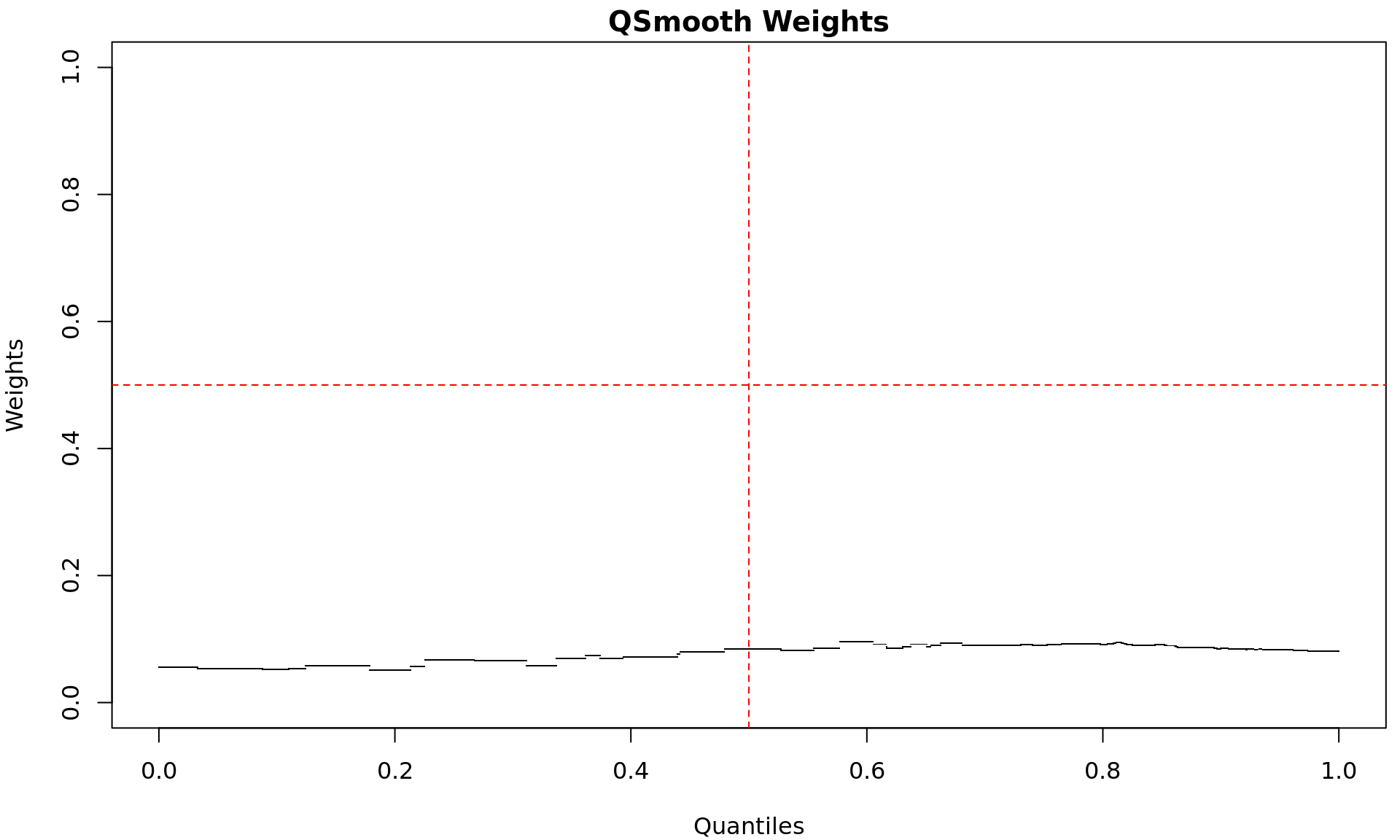
Quantile-specific weights used by the Smooth-Quantile normalisation.
Low weights indicate signal quantiles which appear to be more specific
within a group, whilst higher weights indicate similarity between
groups.
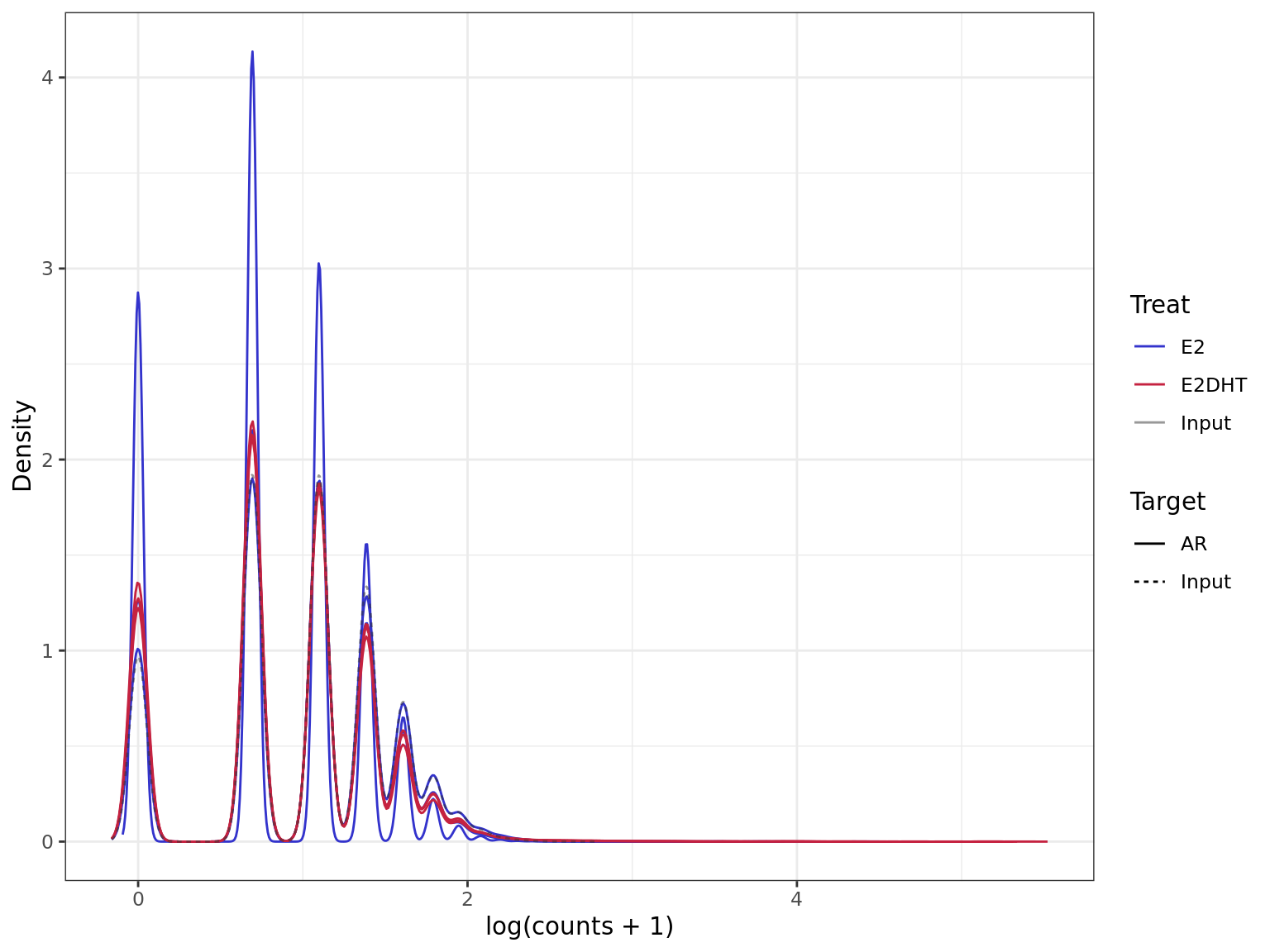
Density plot for all windows prior to the selection of
windows more likely to contain true signal. Retained windows
will be those at the upper end, whilst discarded windows will be at the
lower end.
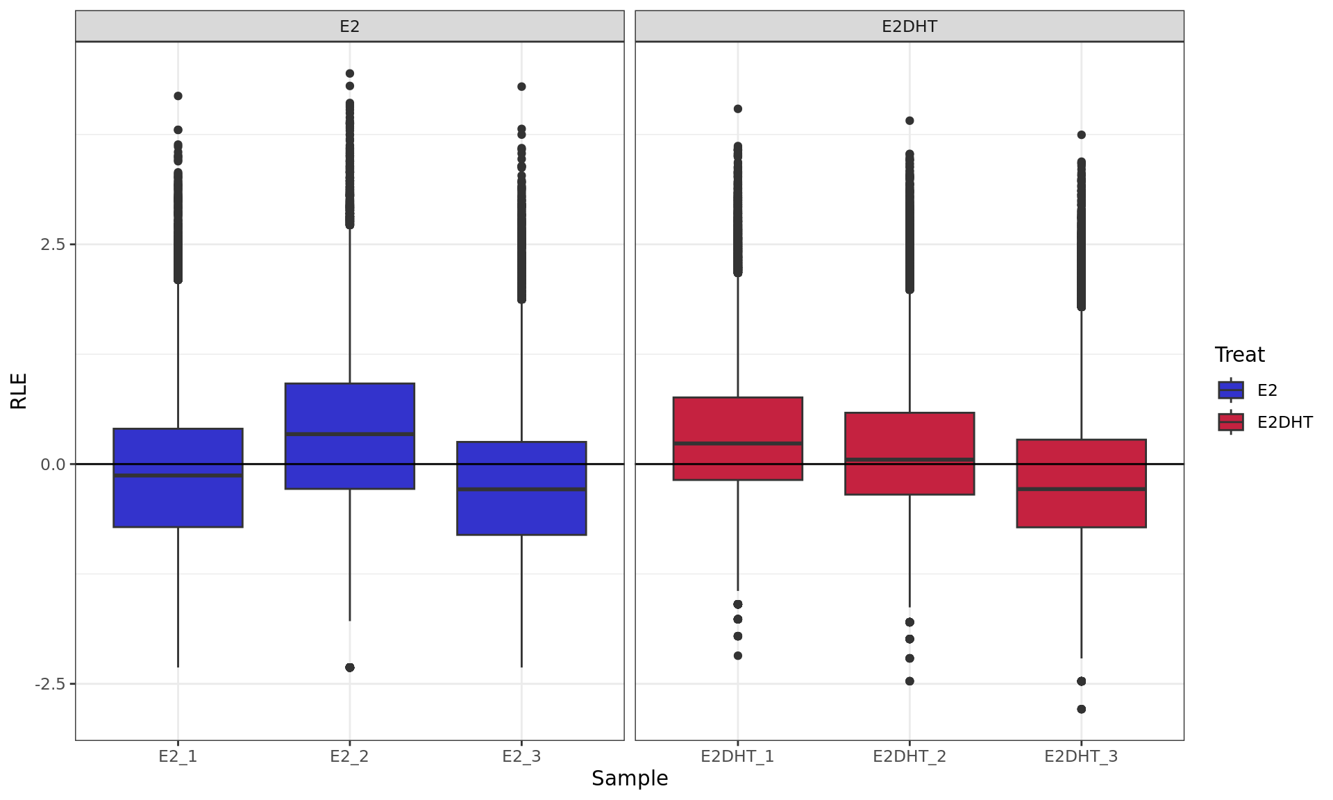
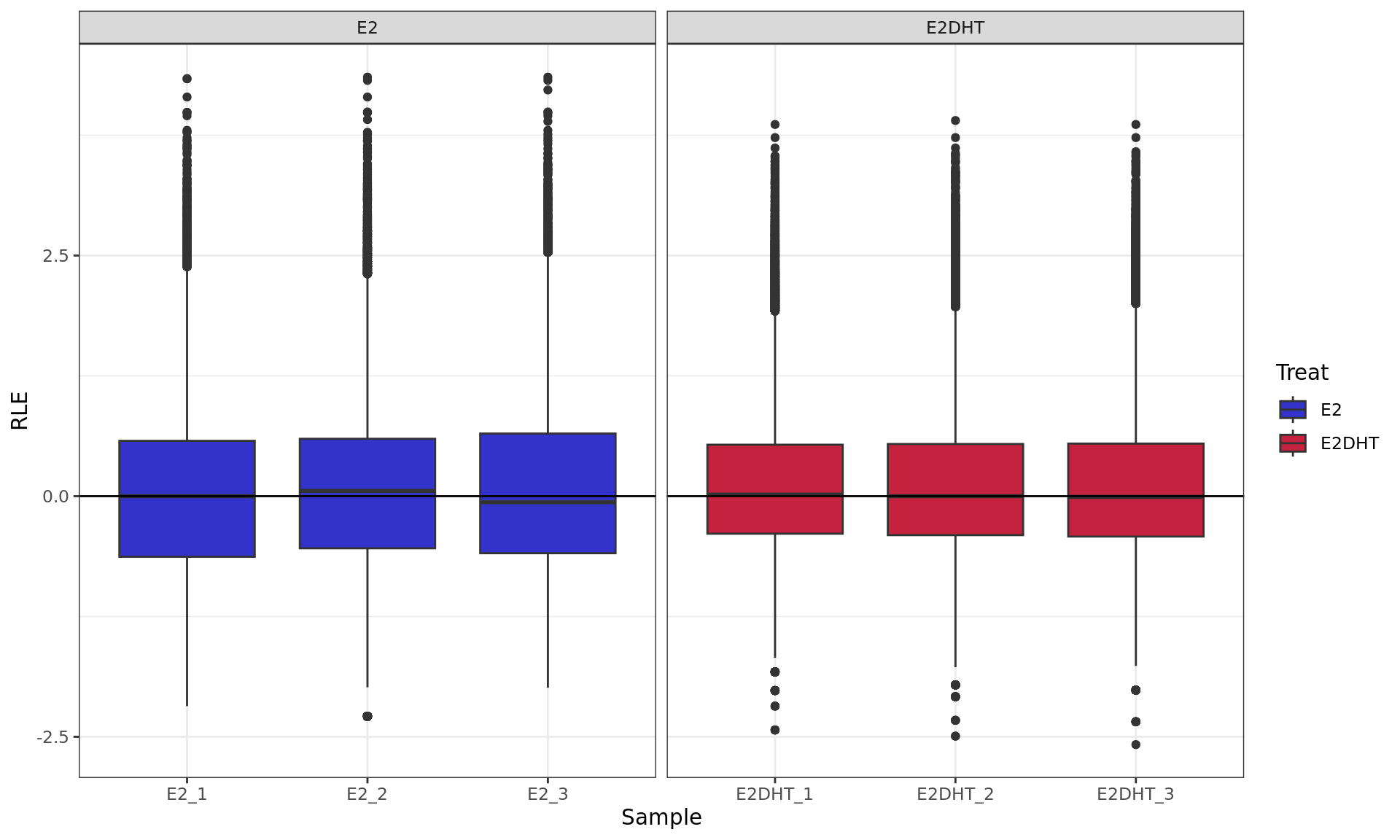
RLE plot showing logCPM values. RLE values were calculated within
each treatment group to account for the potentially different binding
dynamics of AR.
RLE plot showing normalised logCPM. RLE values were calculated
within each treatment group to account for the potentially different
binding dynamics of AR.
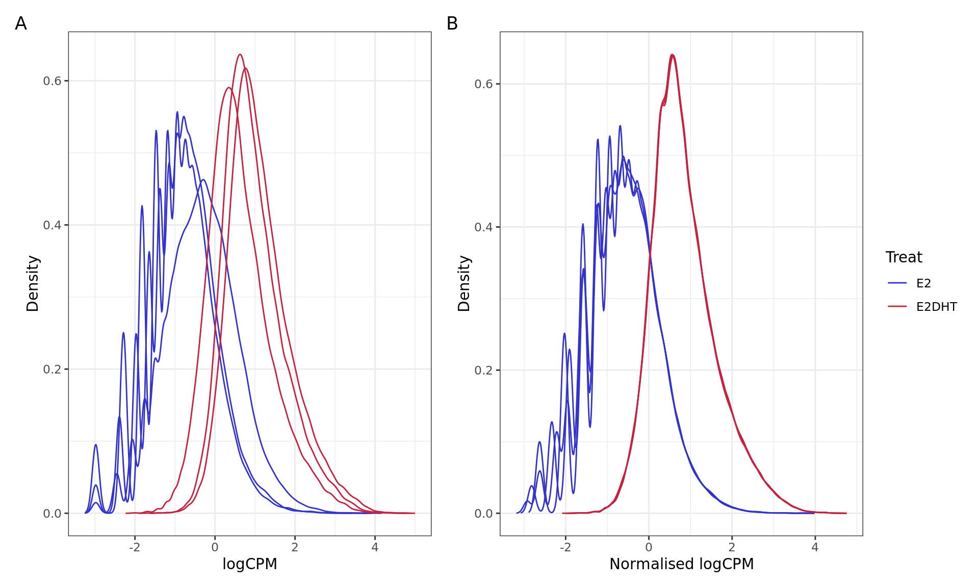
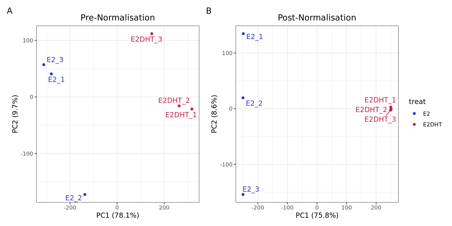
PCA plots for logCPM values A) before and B) after Smooth Quantile
normalisation
Differential Binding Analysis
Primary Analysis
X <- model.matrix(~treat, data = colData(filtered_counts)) %>%
  set_colnames(str_remove(colnames(.), "treat"))
colData(filtered_counts)$design <- X
paired_cors <- block <- txt <- NULL
if (config$comparisons$paired) {
  block <- colData(filtered_counts)[[rep_col]]
  set.seed(1e6)
  ind <- sample.int(nrow(filtered_counts), n_max, replace = FALSE)
  paired_cors <- duplicateCorrelation(
    object = assay(filtered_counts, "qsmooth")[ind, ],
    design = X,
    block = block
  )$consensus.correlation
  txt <- glue(
    "Data were nested within {{rep_col}} as a potential source of correlation. ",
    "The estimated correlation within replicate samples was $\\hat{\\rho} = {{round(paired_cors, 3)}}$",
    .open = "{{", .close = "}}"
  )
}
fc <- ifelse(is.null(config$comparisons$fc), 1, config$comparisons$fc)
fit <- assay(filtered_counts, "qsmooth") %>%
  lmFit(design = X, block = block, correlation = paired_cors) %>%
  treat(fc = fc, trend = TRUE, robust = FALSE)
fit_mu0 <- assay(filtered_counts, "qsmooth") %>%
  lmFit(design = X, block = block, correlation = paired_cors) %>%
  treat(fc = 1, trend = TRUE, robust = FALSE)
res_cols <- c("logFC", "AveExpr", "t", "P.Value", "fdr")
rowData(filtered_counts) <- rowData(filtered_counts) %>%
  .[!colnames(.) %in% c(res_cols, "p_mu0")] %>%
  cbind(
    fit %>%
      topTable(sort.by = "none", number = Inf) %>%
      as.list %>%
      setNames(res_cols) %>%
      c(
        list(
          p_mu0 = topTable(fit_mu0, sort.by = "none", number = Inf)$P.Value
        )
      )
  )
After SQ-normalisation of logCPM values, the limma-trend
method (Law et al. 2014) was applied to all
retained windows. A simple linear model was fitted taking E2 as the
baseline and estimating the effects of E2DHT on AR binding within each
sliding window, incorporating a trended prior-variance.
After model fitting, hypothesis testing was performed testing:
\[
H_0: -\lambda < \mu < \lambda
\] against \[
H_A: |\mu| > \lambda
\] where \(\mu\) represents the
true mean change in AR binding. The value \(\lambda =\) 0.26 was chosen as this
corresponds to a 20% change in detected signal on the log2
scale. This is known as the treat method (McCarthy and Smyth 2009), and p-values
were obtained for each initial window, before merging adjoining
windows.
For subsequent classification when combining across multiple
differential binding results, an additional p-value testing \(\mu = 0\) was added, however this is not
used for detection of sites showing evidence of altered AR binding.
After selection of the 98,742 sliding windows (120bp), these were
merged into 13,512 genomic regions with size ranging from 120 to 1640bp,
with the median width being 360bp. Representative estimates of
differential binding (i.e. logFC) were taken from the sliding window
with the highest average signal across all samples, within each
set of windows to be merged. Similarly, p-values from the above tests
were also selected from the same sliding window as representative of the
merged region (A. T. Lun and Smyth 2015). The number of
windows showing increased or decreased binding within each merged region
were also included, by counting those within each set of windows with
p-values lower than the selected window. FDR-adjustment was performed
with 9,738 regions (72.1%) showing significance, based on an
FDR-adjusted p-value alone.
Independent Hypothesis Weighting (IHW) (Ignatiadis et al.
2016) was then used to partition the raw p-values for AR
differential binding by the detection of the other ChIP targets under
investigation in this workflow (ER and H3K27ac). The presence of ER and
H3K27ac was defined simply using the union peaks detected under any
treatment by macs2 callpeak, as determined previously. This allows recalculation
of the FDR using weighted p-values instead of raw
p-values. In order for IHW to be a viable strategy, partitions
should be greater than 1000. The provided union peaks were used as
initial partitions in combination, merging the smallest groups below
this size until all partitions were of a suitable size.
Windows were classified as overlapping a peak from a secondary ChIP
target if any section of the window overlapped the secondary
peak.
Summary of changes introduced by IHW for windows considered
as being differentially bound by AR. This corresponds to a nett
change of 0.2% from the initial list.
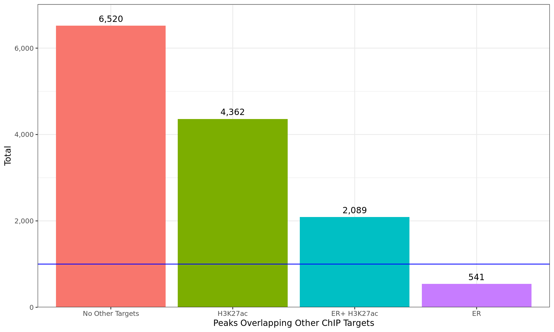
Breakdown of all windows which overlapped peaks from additional ChIP
targets. Any partitions with fewer than 1000 windows (indicated as the
blue horizontal line) were combined into the next smallest partition
consecutively, until all partitions contained > 1000 windows.
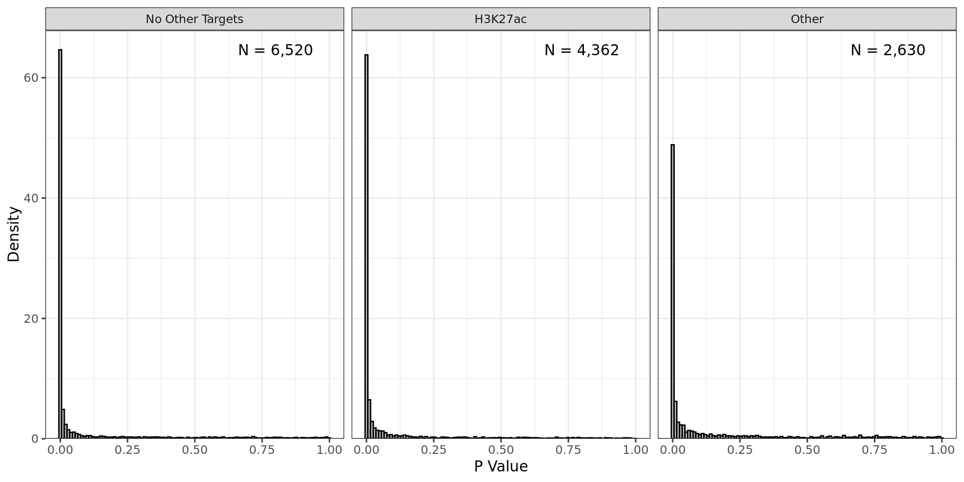
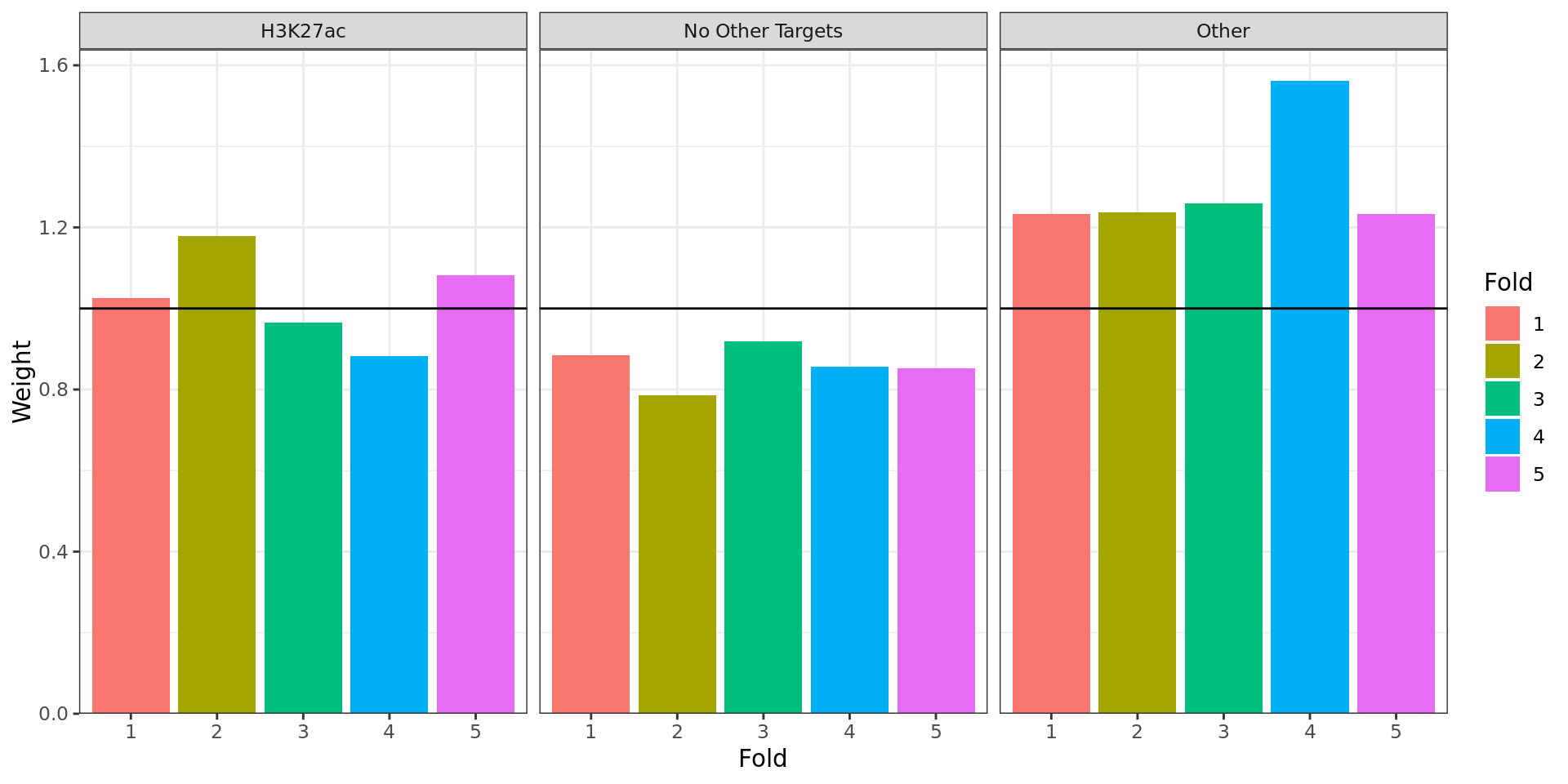
Weights applied to p-values within each partition. ‘Folds’ represent
random sub-partitions within each larger partition generated as part of
the IHW process.
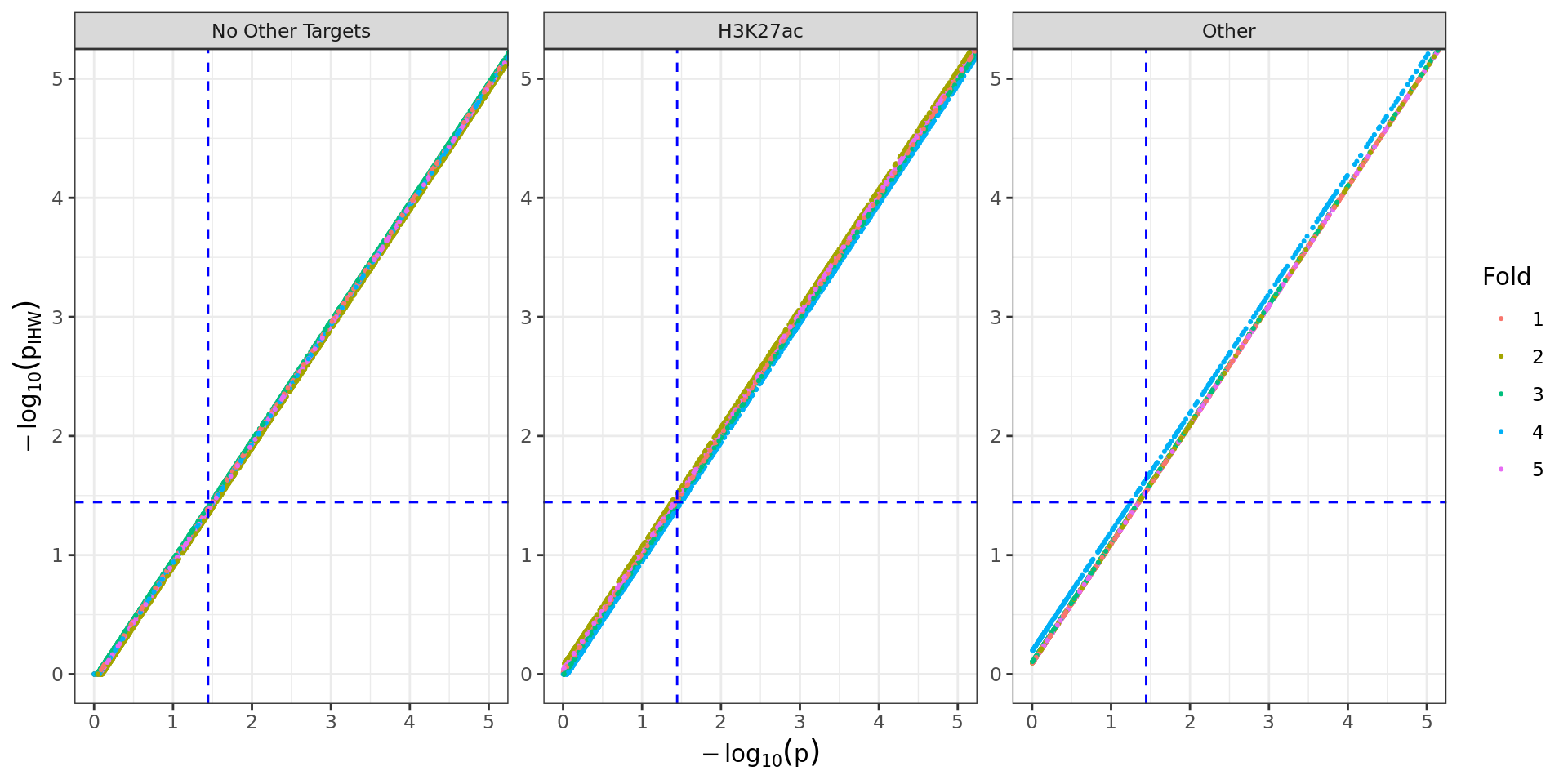
Comparison of raw and weighted p-values for each partition. Blue
dashed lines indicate FDR = 0.05 for each set of p-values. Those in the
lower-right quadrant would no longer be considered significant after
IHW, whilst those in the upper-left quadrant would only be considered as
significant after the IHW process. Those in the upper-right quadrant
would be considered as significant regardless of the methodology.
In addition to statistical analysis, merged windows were first mapped
to the gene-centric region with the largest overlap. Windows were then
mapped to the external features provided in the same manner, followed by
mapping to all annotated genes.
During mapping to genes, promoters were defined the union of all
regions defined based on transcript-level annotation, and any external
features which were defined as promoters. Enhancers were any regions
defined in enhancer_atlas_2.0_zr75.gtf.gz as enhancers.
These features were used to map merged windows to features using the
process defined in the function
extraChIPs::mapByFeature():
Ranges overlapping a promoter are assigned to genes
directly overlapping that specific promoter
Ranges overlapping an enhancer are assigned to all genes
within 100 kb of the enhancer
Ranges overlapping a long-range interaction are assigned to
all genes directly overlapping either end of the interaction
Ranges with no gene assignment from the previous steps are
assigned to all overlapping genes, or the nearest gene within 100kb
Notably, genes are only passed to step 4 if no gene assignment has
been made in steps 1, 2 or 3. For visualisation purposes, only genes
which were considered as detected in any provided RNA-Seq data will be
shown as the mapping targets.
tbl <- merged_results %>%
  mutate(w = width) %>%
  as_tibble() %>%
  group_by(status) %>%
  summarise(
    n = dplyr::n(),
    width = median(w),
    AveExpr = median(AveExpr),
    .groups = "drop"
  ) %>%
  mutate(`%` = n / sum(n)) %>%
  dplyr::select(status, n, `%`, everything()) %>%
  reactable(
    searchable = FALSE, filterable = FALSE,
    columns = list(
      status = colDef(
        name = "Status", maxWidth = 150,
        footer = htmltools::tags$b("Overall")
      ),
      n = colDef(
        name = "Nbr of Windows", maxWidth = 150, format = colFormat(separators = TRUE),
        footer = htmltools::tags$b(comma(length(merged_results)))
      ),
      width = colDef(
        name = "Median Width (bp)", format = colFormat(digits = 1),
        footer = htmltools::tags$b(round(median(width(merged_results)), 1)),
        maxWidth = 200
      ),
      `%` = colDef(
        name = "% Total Windows", format = colFormat(percent = TRUE, digits = 1),
        style = function(value) bar_style(width = value, align = "right"),
        maxWidth = 150
      ),
      AveExpr = colDef(
        name = "Median Signal (logCPM)",
        format = colFormat(digits = 3),
        maxWidth = 200,
        footer = htmltools::tags$b(
          round(median(merged_results$AveExpr), 3)
        )
      )
    )
  )
cp <- htmltools::em(
  glue(
    "Overall results for changed {target} binding in the ",
    glue_collapse(rev(treat_levels), last = " Vs. "),
    " comparison."
  )
)
div(class = "table",
  div(class = "table-header",
      div(class = "caption", cp),
      tbl
  )
)
Overall results for changed AR binding in the E2DHT Vs. E2 comparison.
Summary By Region
df <- merged_results %>%
  select(
    status, all_of(fdr_column), region
  ) %>%
  as_tibble() %>%
  group_by(region, status) %>%
  summarise(n = dplyr::n(), .groups = "drop") %>%
  complete(region, status, fill = list(n = 0)) %>%
  group_by(region) %>%
  mutate(Total = sum(n)) %>%
  ungroup() %>%
  pivot_wider(names_from = "status", values_from = "n") %>%
  mutate(
    `% Of All Windows` = Total / length(merged_results),
    `% Changed` = 1 - Unchanged / Total
  ) %>%
  arrange(region) %>%
  dplyr::select(
    Region = region,
    any_of(names(direction_colours)),
    `% Changed`, Total, `% Of All Windows`
  )
cp <- htmltools::em(
  glue(
    "Overall results for changed {target} binding in the ",
    glue_collapse(rev(treat_levels), last = " Vs. "),
    " comparison, broken down by which genomic region contains the largest ",
    "overlap with each merged window."
  )
)
tbl <- df %>%
  reactable(
    columns = tbl_cols[colnames(df)],
    defaultColDef = colDef(
      footer = function(values) htmltools::tags$b(comma(sum(values)))
    ),
    fullWidth = TRUE
  )
div(class = "table",
  div(class = "table-header",
      div(class = "caption", cp),
      tbl
  )
)
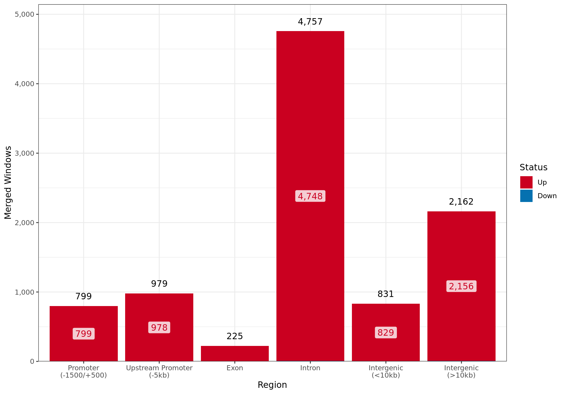
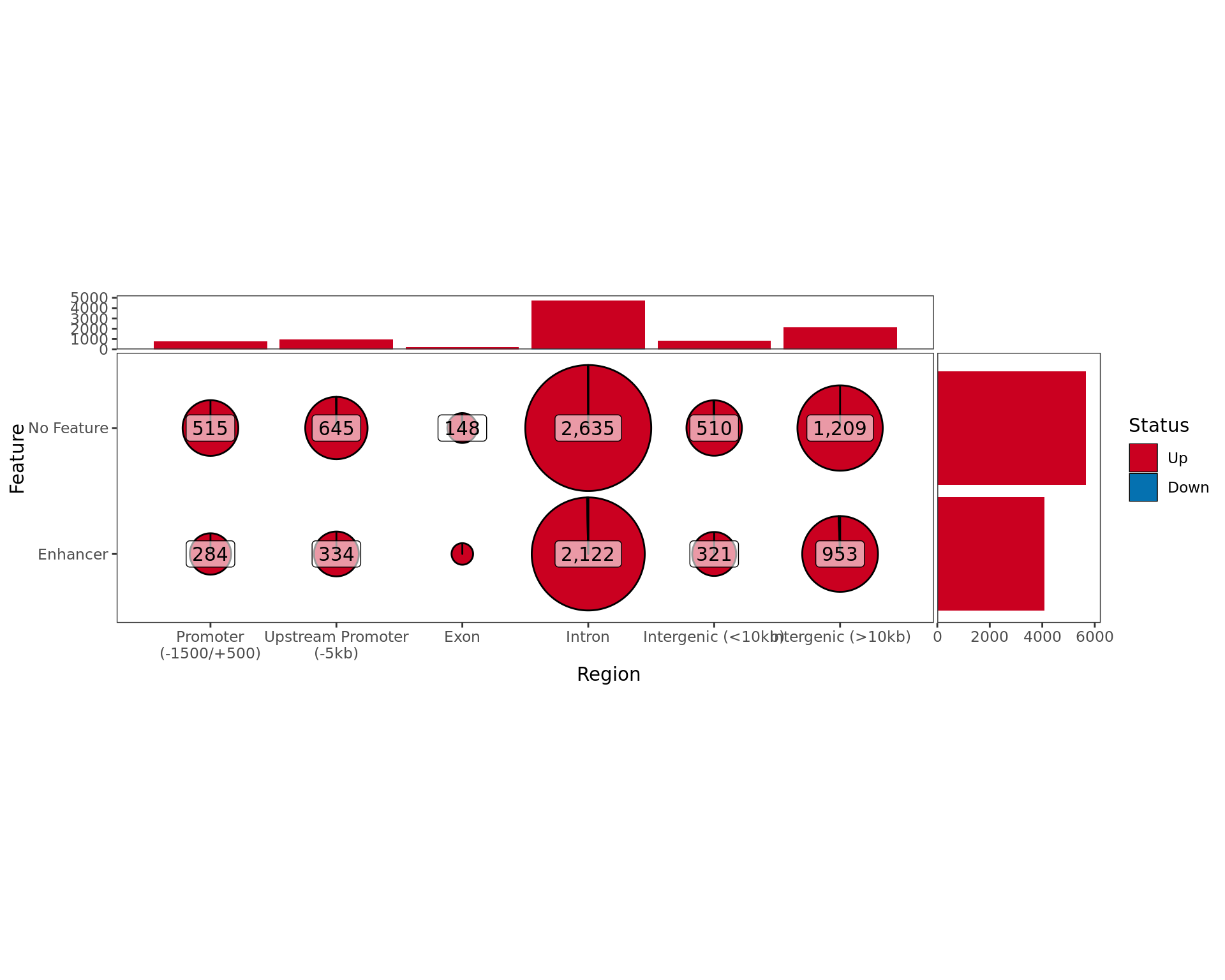
Overall results for changed AR binding in the E2DHT Vs. E2 comparison, broken down by which genomic region contains the largest overlap with each merged window.
Summary By Feature
df <- merged_results %>%
  select(status, all_of(fdr_column), feature) %>%
  as_tibble() %>%
  group_by(feature, status) %>%
  tally() %>%
  ungroup() %>%
  complete(feature, status, fill = list(n = 0)) %>%
  group_by(feature) %>%
  mutate(Total = sum(n)) %>%
  ungroup() %>%
  pivot_wider(names_from = "status", values_from = "n") %>%
  mutate(
    `% Of All Windows` = Total / length(merged_results),
    `% Changed` = 1 - Unchanged / Total
  ) %>%
  arrange(feature) %>%
  dplyr::select(
    Feature = feature,
    any_of(names(direction_colours)),
    `% Changed`, Total, `% Of All Windows`
  )
cp <- htmltools::em(
  glue(
    "Overall results for changed {target} binding in the ",
    glue_collapse(rev(treat_levels), last = " Vs. "),
    " comparison, broken down by which external feature contains the largest ",
    "overlap with each merged window."
  )
)
tbl <- df %>%
  reactable(
    columns = tbl_cols[colnames(df)],
    defaultColDef = colDef(
      footer = function(values) htmltools::tags$b(comma(sum(values)))
    )
  )
div(class = "table",
  div(class = "table-header",
      div(class = "caption", cp),
      tbl
  )
)
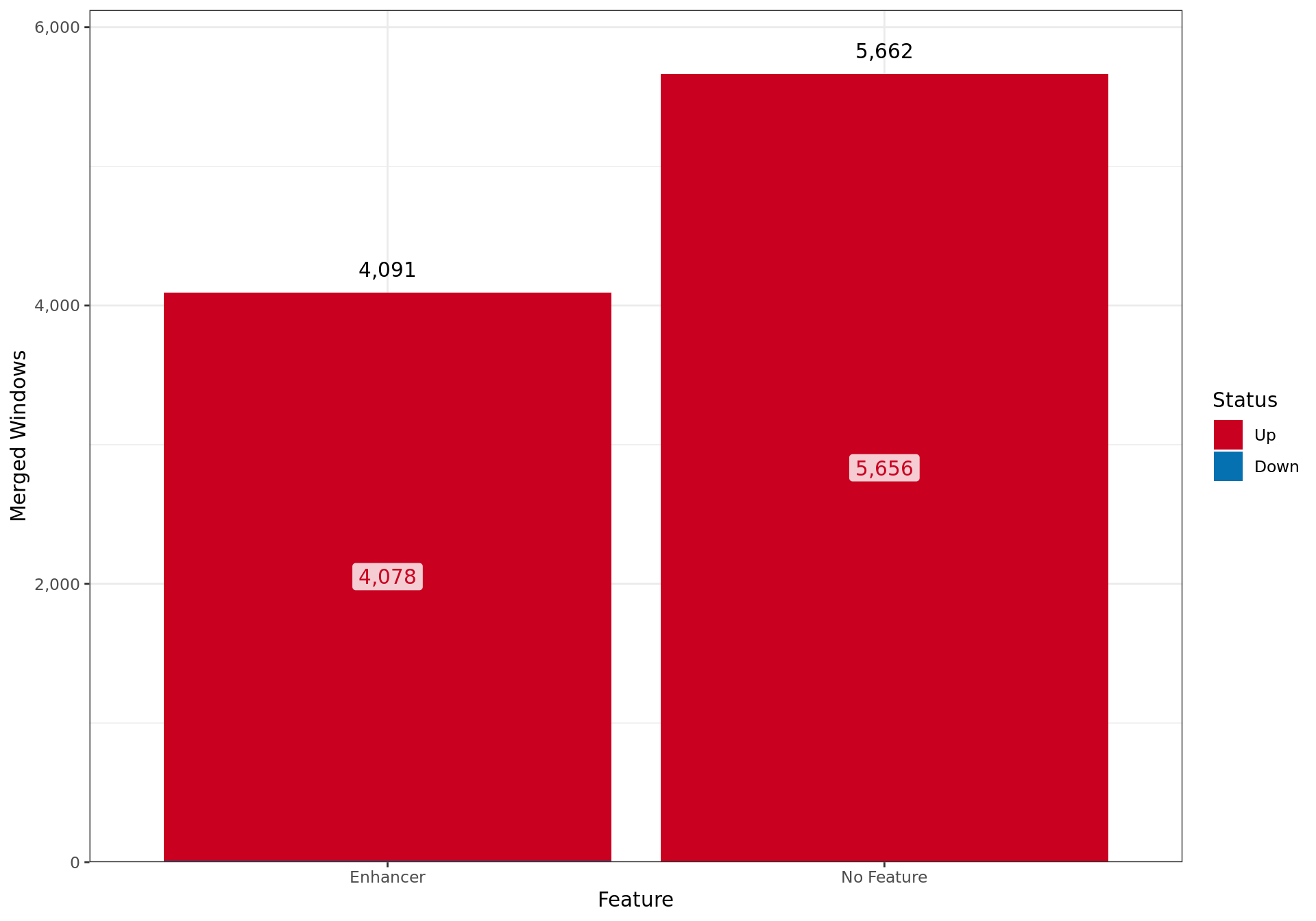
Overall results for changed AR binding in the E2DHT Vs. E2 comparison, broken down by which external feature contains the largest overlap with each merged window.
Most Highly Ranked
show_n <- min(200, length(merged_results))
scaling_vals <- list(
  logFC = c(-1, 1)*max(abs(merged_results$logFC)),
  AveExpr = range(merged_results$AveExpr),
  Width = max(width(merged_results))
)
cp <- htmltools::em(
  glue(
    "The {show_n} most highly-ranked windows by FDR, with ",
    sum(merged_results$P.Value_fdr < fdr_alpha),
    " showing evidence of changed {target} binding. ",
    "Regions were assigned based on which genomic region showed the largest ",
    "overlap with the final merged window. ",
    ifelse(
      has_features,
      glue("Features are as provided in the file {basename(config$external$features)}. "),
      glue("")
    ),
    "For windows mapped to large numbers of genes, hovering a mouse over the ",
    "cell will reveal the full set of genes. ",
    ifelse(
      has_rnaseq,
      "Only genes considered as detected in the RNA-Seq data are shown. ",
      ""
    ),
    "The Macs2 Peak column is filterable using T/F values"
  )
)
fs <- 12
tbl <- merged_results %>%
  mutate(w = width) %>%
  arrange(!!sym(fdr_column)) %>%
  plyranges::slice(seq_len(show_n)) %>%
  select(
    w, AveExpr, logFC, FDR = !!sym(fdr_column),
    overlaps_ref, Region = region, any_of("feature"), Genes = gene_name
  ) %>%
  as_tibble() %>%
  dplyr::rename(
    Range = range, `Width (bp)` = w, `Macs2 Peak` = overlaps_ref
  ) %>%
  rename_all(str_replace_all, "feature", "Feature") %>%
  mutate(Genes = vapply(Genes, paste, character(1), collapse = "; ")) %>%
  reactable(
    filterable = TRUE,
    showPageSizeOptions = TRUE,
    pageSizeOptions = c(10, 20, 50, show_n), defaultPageSize = 10,
    borderless  = TRUE,
    columns = list(
      Range = colDef(
        minWidth = 10 * fs,
        cell = function(value) {
          str_replace_all(value, ":", ": ")
        }
      ),
      `Width (bp)` = colDef(
        style = function(value) {
          x <- value / scaling_vals$Width
          colour <- expr_col(x)
          list(
            background = colour,
            borderRight = "1px solid rgba(0, 0, 0, 0.1)"
          )
        },
        maxWidth = 5 * fs
      ),
      AveExpr = colDef(
        cell = function(value) round(value, 2),
        style = function(value) {
          x <- (value - min(scaling_vals$AveExpr)) / diff(scaling_vals$AveExpr)
          colour = expr_col(x)
          list(background = colour)
        },
        maxWidth = 5.5 * fs
      ),
      logFC = colDef(
        cell = function(value) round(value, 2),
        style = function(value) {
          x <- (value - min(scaling_vals$logFC)) / diff(scaling_vals$logFC)
          colour <- lfc_col(x)
          list(background = colour)
        },
        maxWidth = 5.5 * fs
      ),
      FDR = colDef(
        cell = function(value) sprintf("%.2e", value),
        style = list(borderRight = "1px solid rgba(0, 0, 0, 0.1)"),
        maxWidth = 5.5 * fs
      ),
      `Macs2 Peak` = colDef(
        cell = function(value) ifelse(value, "\u2714 Yes", "\u2716 No"),
        style = function(value) {
          color <- ifelse(value, "#008000", "#e00000")
          list(color = color, borderRight = "1px solid rgba(0, 0, 0, 0.1)")
        },
        maxWidth = 5 * fs
      ),
      Region = colDef(maxWidth = 150),
      Genes = colDef(
        cell = function(value) with_tooltip(value),
        minWidth = 11 * fs
      )
    ),
    theme = reactableTheme(style = list(fontSize = fs))
  )
div(class = "table",
  div(class = "table-header",
      div(class = "caption", cp),
      tbl
  )
)
The 200 most highly-ranked windows by FDR, with 9738 showing evidence of changed AR binding. Regions were assigned based on which genomic region showed the largest overlap with the final merged window. Features are as provided in the file enhancer_atlas_2.0_zr75.gtf.gz. For windows mapped to large numbers of genes, hovering a mouse over the cell will reveal the full set of genes. Only genes considered as detected in the RNA-Seq data are shown. The Macs2 Peak column is filterable using T/F values
Summary Plots
profile_width <- 5e3
n_bins <- 100
bwfl <- file.path(
    macs2_path, glue("{target}_{treat_levels}_merged_treat_pileup.bw")
  ) %>%
  BigWigFileList() %>%
  setNames(treat_levels)
sig_ranges <- merged_results %>%
  filter(!!sym(fdr_column) < fdr_alpha) %>%
  colToRanges("keyval_range") %>%
  splitAsList(f = .$direction) %>%
  .[vapply(., length, integer(1)) > 0]
fc_heat <- names(sig_ranges) %>%
  lapply(
    function(x) {
      glue(
        "
        *Heatmap and histogram for all regions considered to show evidence of
        {ifelse(x == 'Up', 'increased', 'decreased')} {target} binding in
        response to {treat_levels[[2]]} treatment. A total of
        {comma(length(sig_ranges[[x]]))} regions were in this group.
        ",
        ifelse(
          length(sig_ranges[[x]]) > 2e4,
          " Due to the large number of regions, these were randomly down-sampled to 20,000 for viable plotting.",
          ""
        ),
        "*"
      )
    }
  ) %>%
  setNames(names(sig_ranges))
sig_profiles <- lapply(sig_ranges, function(x) NULL)
for (i in names(sig_profiles)) {
  ## Restrict to 20,000. Plots work poorly above this number.
  ## Randomly sample
  set.seed(threads)
  temp_gr <- granges(sig_ranges[[i]])
  n <- length(temp_gr)
  if (n > 2e4) temp_gr <- temp_gr[sort(sample.int(n, 2e4))]
  sig_profiles[[i]] <- getProfileData(
    bwfl, temp_gr, upstream = profile_width / 2, bins = n_bins,
    BPPARAM = bpparam()
  )
  rm(temp_gr)
}
profile_heatmaps <- sig_profiles %>%
  parallel::mclapply(
    plotProfileHeatmap,
    profileCol = "profile_data",
    colour = "name",
    xLab = "Distance from Centre (bp)",
    fillLab = "logCPM",
    mc.cores = length(sig_profiles)
  )
fill_range <- profile_heatmaps %>%
  lapply(function(x) x$data[,"score"]) %>%
  unlist() %>%
  range()
sidey_range <- profile_heatmaps %>%
  lapply(function(x) x$layers[[3]]$data$y) %>%
  unlist() %>%
  range()
profile_heatmaps <- profile_heatmaps %>%
  lapply(
    function(x) {
      suppressWarnings(
        x +
          scale_fill_gradientn(colours = colours$heatmaps, limits = fill_range) +
          scale_xsidey_continuous(limits = sidey_range) +
          scale_colour_manual(values = treat_colours) +
          labs(
            x = "Distance from Centre (bp)",
            fill = "logCPM",
            colour = "Treat"
          ) +
          theme(
            strip.text.y = element_text(angle = 0)
          )
      )
    }
  )
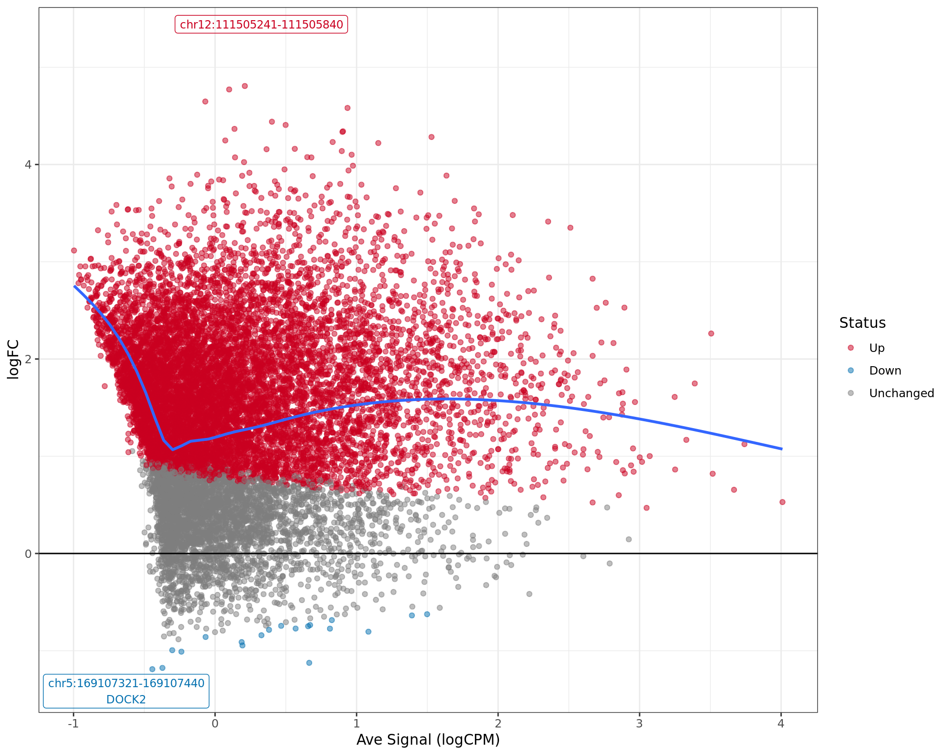
MA plot showing the status of each window under consideration. The
two most extreme regions are labelled by region and any associated
genes, whilst the overall pattern of association between signal level
(logCPM) and changed signal (logFC) is shown as the blue curve.
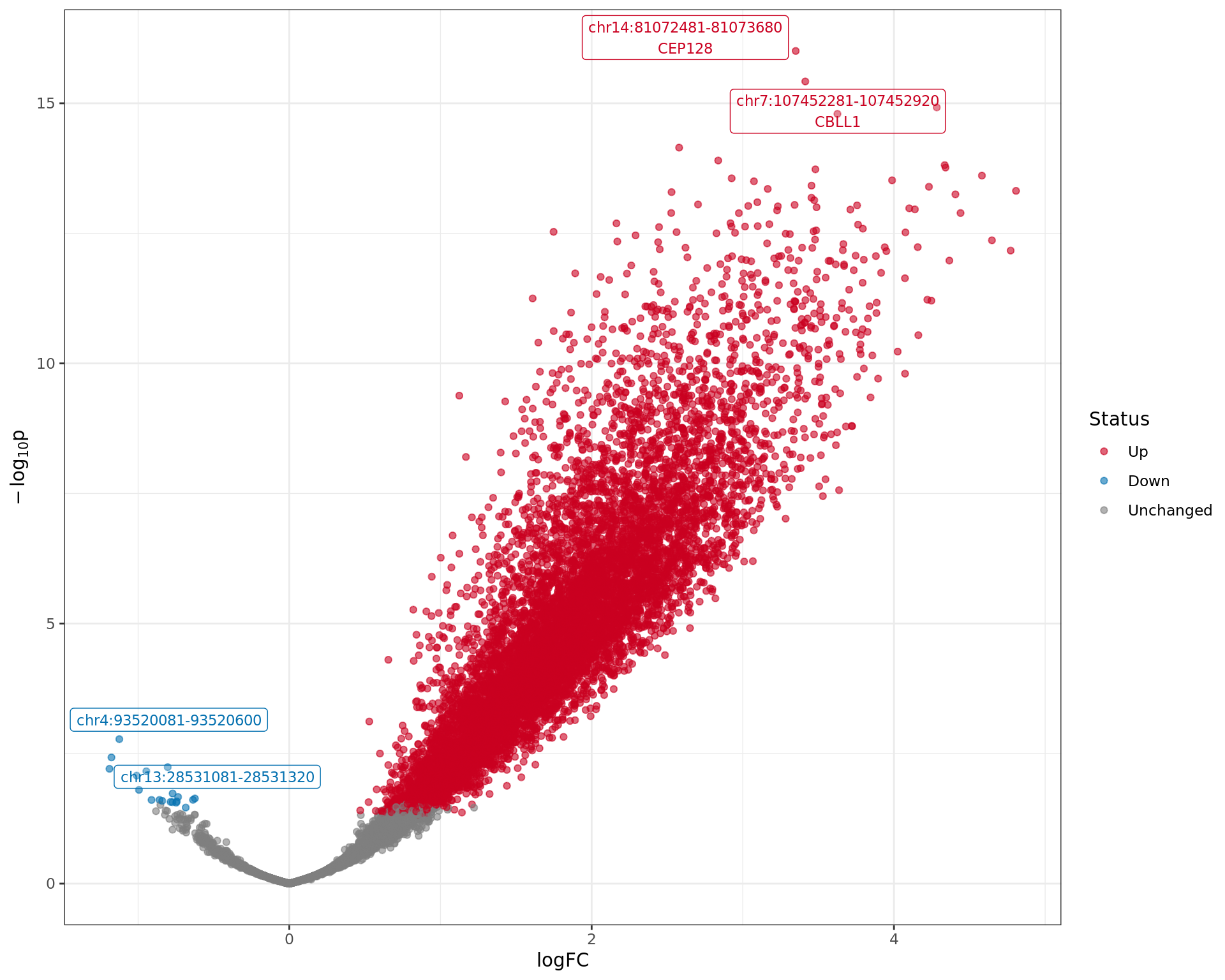
Volcano plot showing regions with evidence of differential AR
binding. The most significant regions are labelled along with any genes
these regions are mapped to.
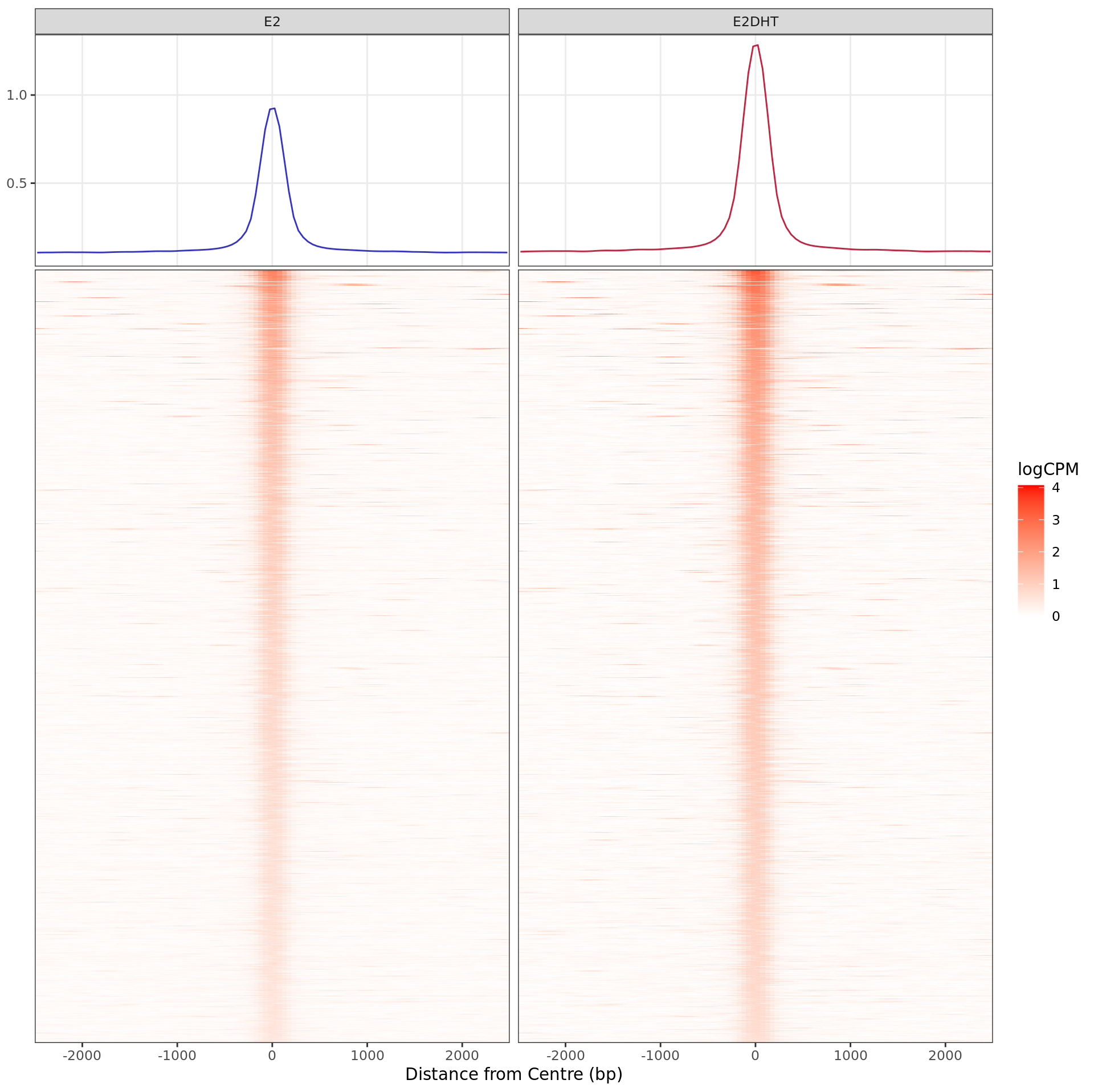
Heatmap: Increased Binding
profile_heatmaps$Up + guides(colour = "none")
Heatmap and histogram for all regions considered to show evidence of
increased AR binding in response to E2DHT treatment. A total of 9,734
regions were in this group.
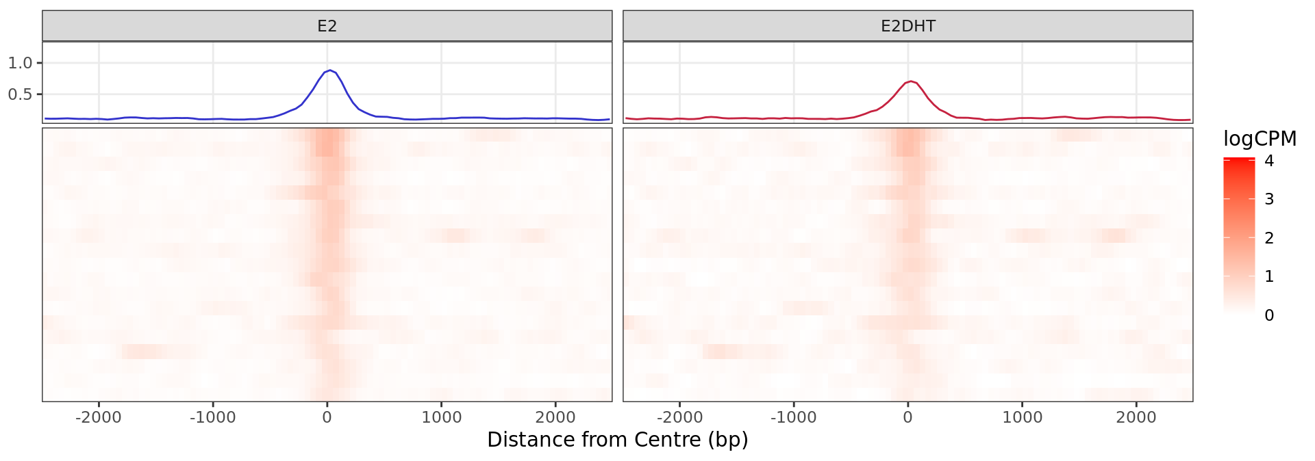
Heatmap: Decreased Binding
profile_heatmaps$Down + guides(colour = "none")
Heatmap and histogram for all regions considered to show evidence of
decreased AR binding in response to E2DHT treatment. A total of 19
regions were in this group.
Results By Chromosome
merged_results %>%
  select(status) %>%
  as.data.frame() %>%
  mutate(
    merge_status = fct_collapse(
      status,
      Up = "Up",
      Down = "Down",
      `Ambiguous/Unchanged` = intersect(c("Ambiguous", "Unchanged"), levels(status))
    )
  ) %>%
  ggplot(aes(seqnames, fill = status)) +
  geom_bar() +
  facet_grid(merge_status~., scales = "free_y") +
  scale_y_continuous(expand = expansion(c(0, 0.05)), labels = comma) +
  scale_fill_manual(values =  direction_colours) +
  labs(
    x = "Chromosome", y = "Number of Windows",
    fill = "Status", alpha = "Macs2 Peak"
  )
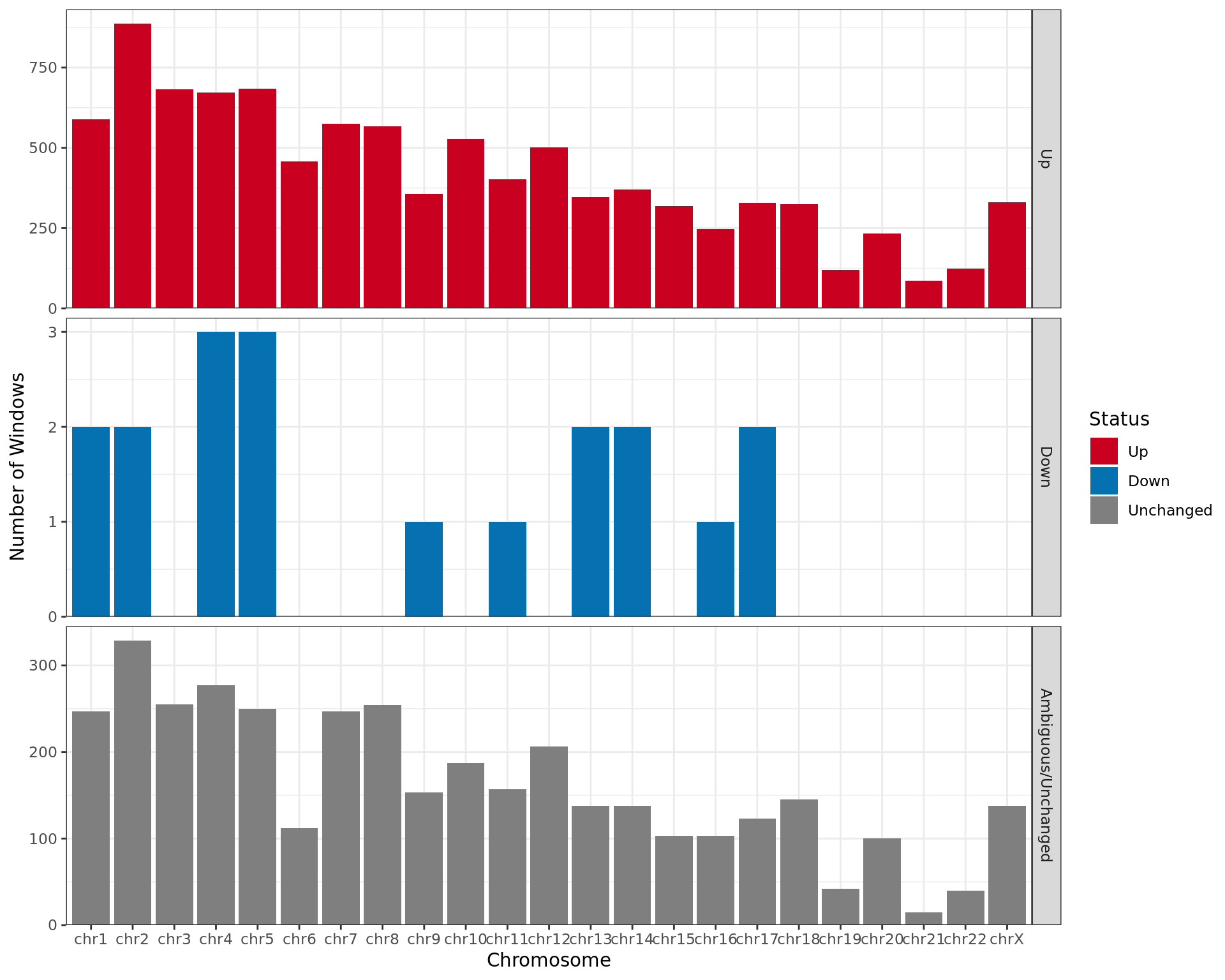
Results for differential binding separated by chromosome
makeCaption <- function(.gr) {
  if (is.null(.gr)) return(NULL)
  dir <- ifelse(.gr$direction == "Down", 'decreased', 'increased')
  reg <- case_when(
    str_detect(.gr$region, "Inter") ~ paste("an", .gr$region, "region"),
    str_detect(.gr$region, "Upstream") ~ paste("an", .gr$region),
    str_detect(.gr$region, "(Ex|Intr)on") ~ paste("an", .gr$region),
    str_detect(.gr$region, "^Prom") ~ paste("a", .gr$region)
  )
  feat <- c()
  if (has_features) feat <- case_when(
    str_detect(.gr$feature, "^[AEIOU]") ~ paste("an", .gr$feature),
    !str_detect(.gr$feature, "^[AEIOU]") ~ paste("a", .gr$feature)
  )
  gn <- unlist(.gr$gene_name)
  fdr <- mcols(.gr)[[fdr_column]]
  fdr <- ifelse(
    fdr < 0.001, sprintf('%.2e', fdr), sprintf('%.3f', fdr)
  )
  cp <- c(
    glue(
      "*The {width(.gr)}bp region showing {dir} {target} binding in response to ",
      "{treat_levels[[2]]} treatment (FDR = {fdr}). ",
      "The range mostly overlapped with {reg}, with all ",
      "defined regions shown as a contiguous bar. ",
      ifelse(
        has_features,
        glue(
          "Using the features supplied in {basename(config$external$features)}, ",
          "this mostly overlapped {feat}, shown as a separate block ",
          "with the gene-centric regions. "
        ),
        glue("")
      ),
    ),
    ifelse(
      .gr$overlaps_ref,
      paste(
        "A union peak overlapping this region was identified by",
        "`macs2 callpeak` when using merged samples."
      ),
      "No union peak was identified using `macs2 callpeak`."
    ),
    ifelse(
      length(gn) > 0,
      paste0(
        "Using the above mapping strategy, this range is likely to regulate ",
        collapseGenes(gn, format = "")
      ),
      "No genes were able to be assigned to this region."
    ),
    paste(
      "For each sample, the y-axis limits represent the values from the window",
      "with the highest signal.*"
    )
  )
  paste(cp, collapse = " ")
}
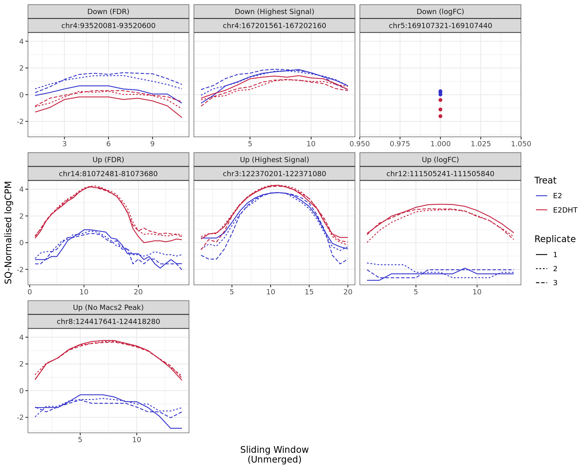
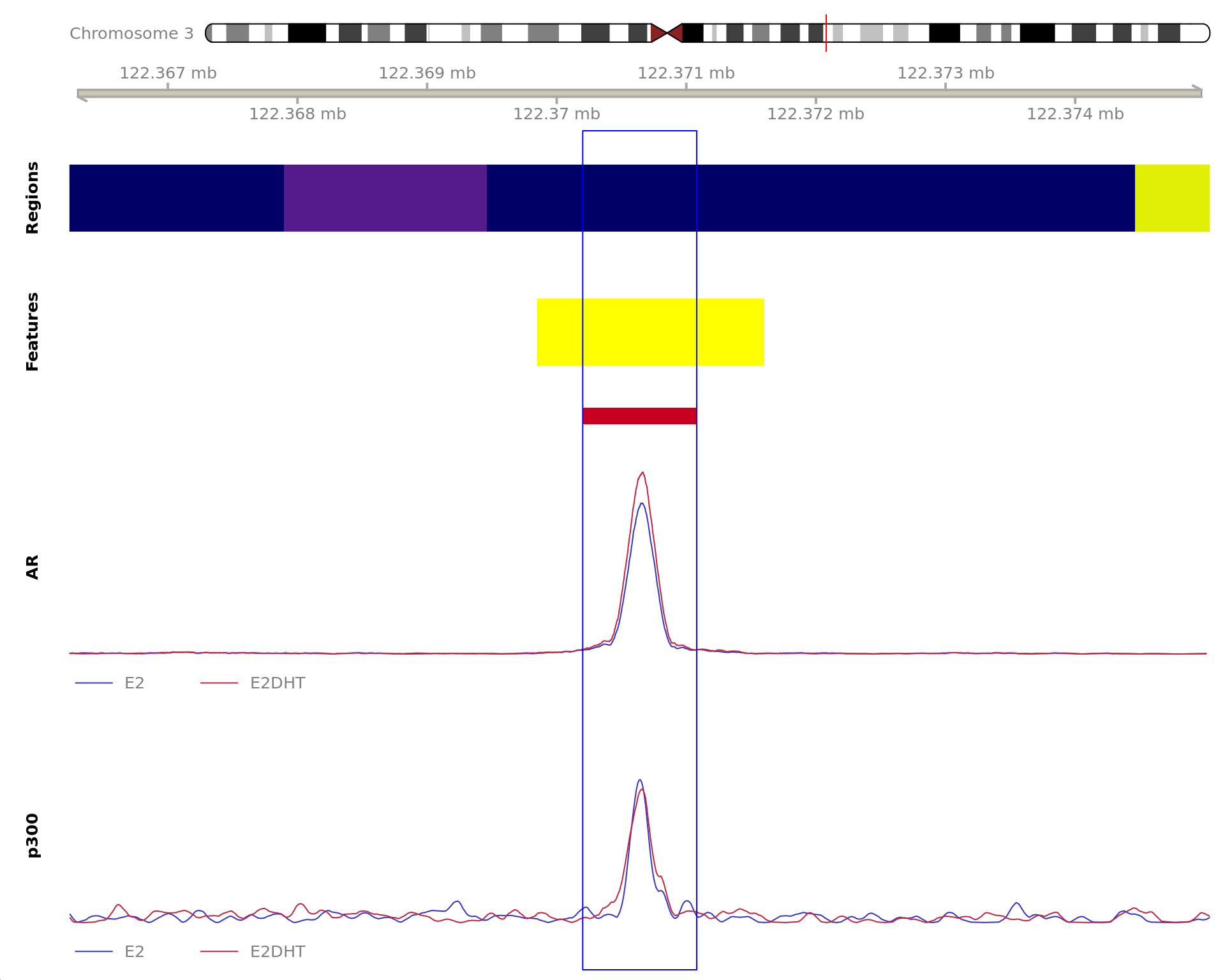
Most highly ranked ranges for both gained and decreased AR binding
in repsonse to E2DHT treatment. The smooth-quantile normalised values
are shown across the initial set of sliding windows before merging.
Ranges were chosen as the most extreme for FDR, Binding Strength
(Signal) and logFC. Windows are shown free of the genomic context.
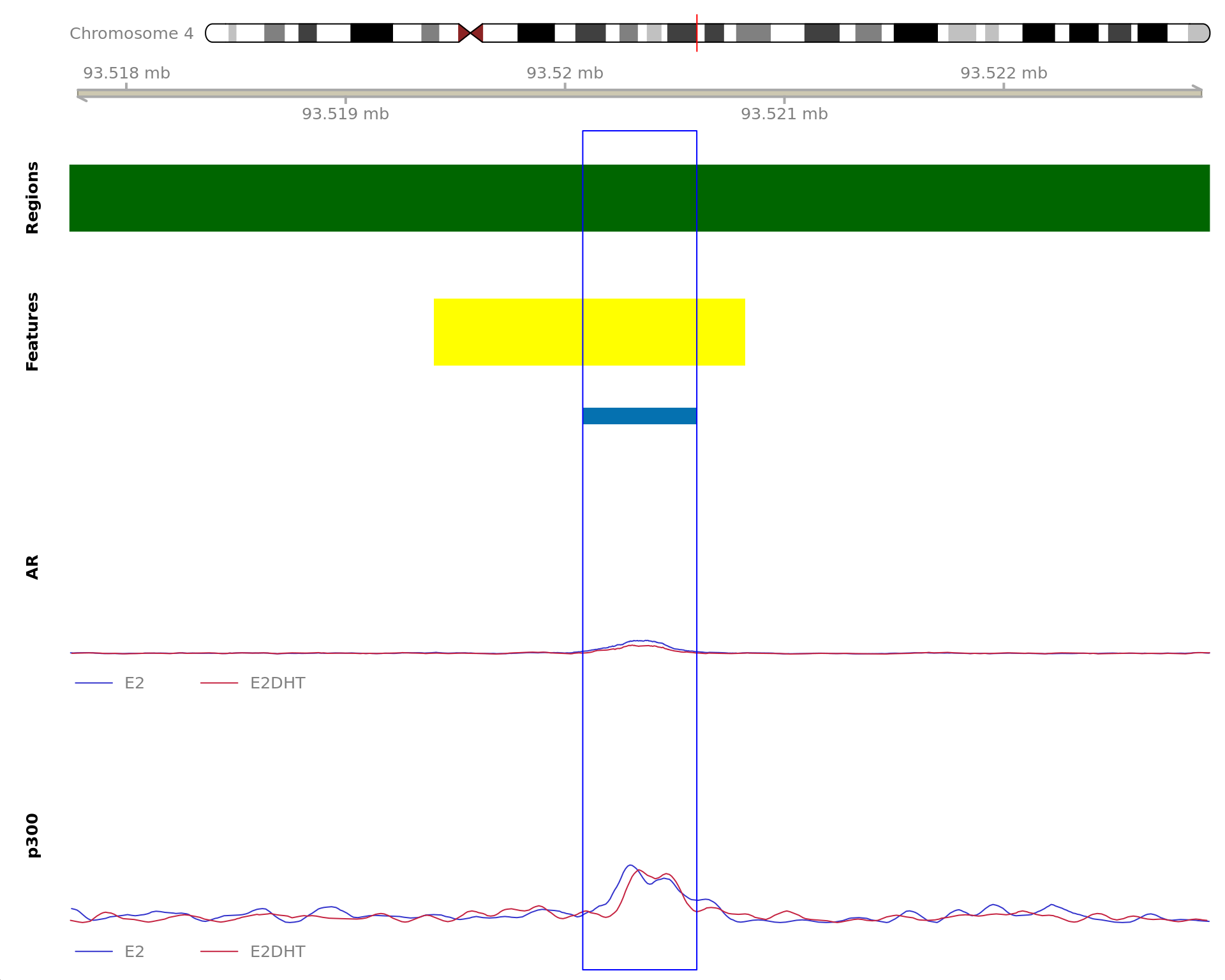
The 600bp region showing decreased AR binding in response to E2DHT
treatment (FDR = 0.038). The range mostly overlapped with an Intergenic
(>10kb) region, with all defined regions shown as a contiguous bar.
Using the features supplied in enhancer_atlas_2.0_zr75.gtf.gz, this
mostly overlapped an Enhancer, shown as a separate block with the
gene-centric regions. A union peak overlapping this region was
identified by macs2 callpeak when using merged samples. No
genes were able to be assigned to this region. For each sample, the
y-axis limits represent the values from the window with the highest
signal.
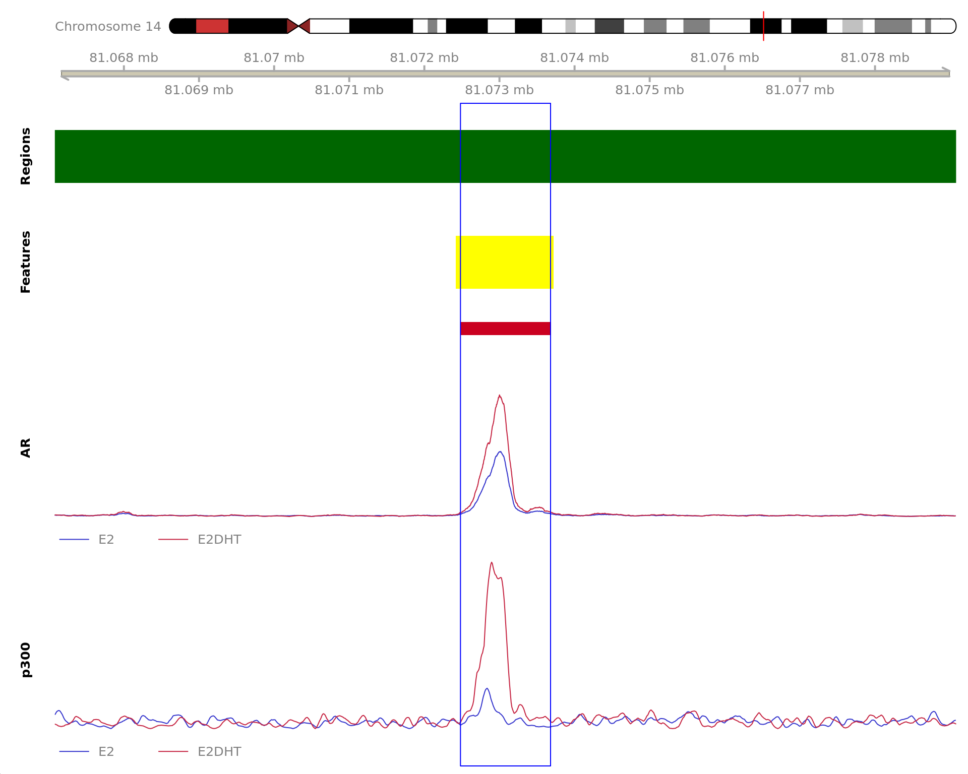
The 520bp region showing decreased AR binding in response to E2DHT
treatment (FDR = 0.003). The range mostly overlapped with an Intron,
with all defined regions shown as a contiguous bar. Using the features
supplied in enhancer_atlas_2.0_zr75.gtf.gz, this mostly overlapped an
Enhancer, shown as a separate block with the gene-centric regions. A
union peak overlapping this region was identified by
macs2 callpeak when using merged samples. No genes were
able to be assigned to this region. For each sample, the y-axis limits
represent the values from the window with the highest signal.
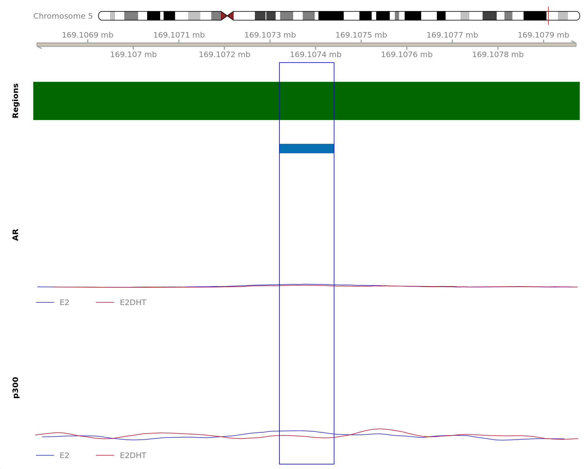
The 120bp region showing decreased AR binding in response to E2DHT
treatment (FDR = 0.011). The range mostly overlapped with an Intron,
with all defined regions shown as a contiguous bar. Using the features
supplied in enhancer_atlas_2.0_zr75.gtf.gz, this mostly overlapped a No
Feature, shown as a separate block with the gene-centric regions. No
union peak was identified using macs2 callpeak. Using the
above mapping strategy, this range is likely to regulate DOCK2 For each
sample, the y-axis limits represent the values from the window with the
highest signal.
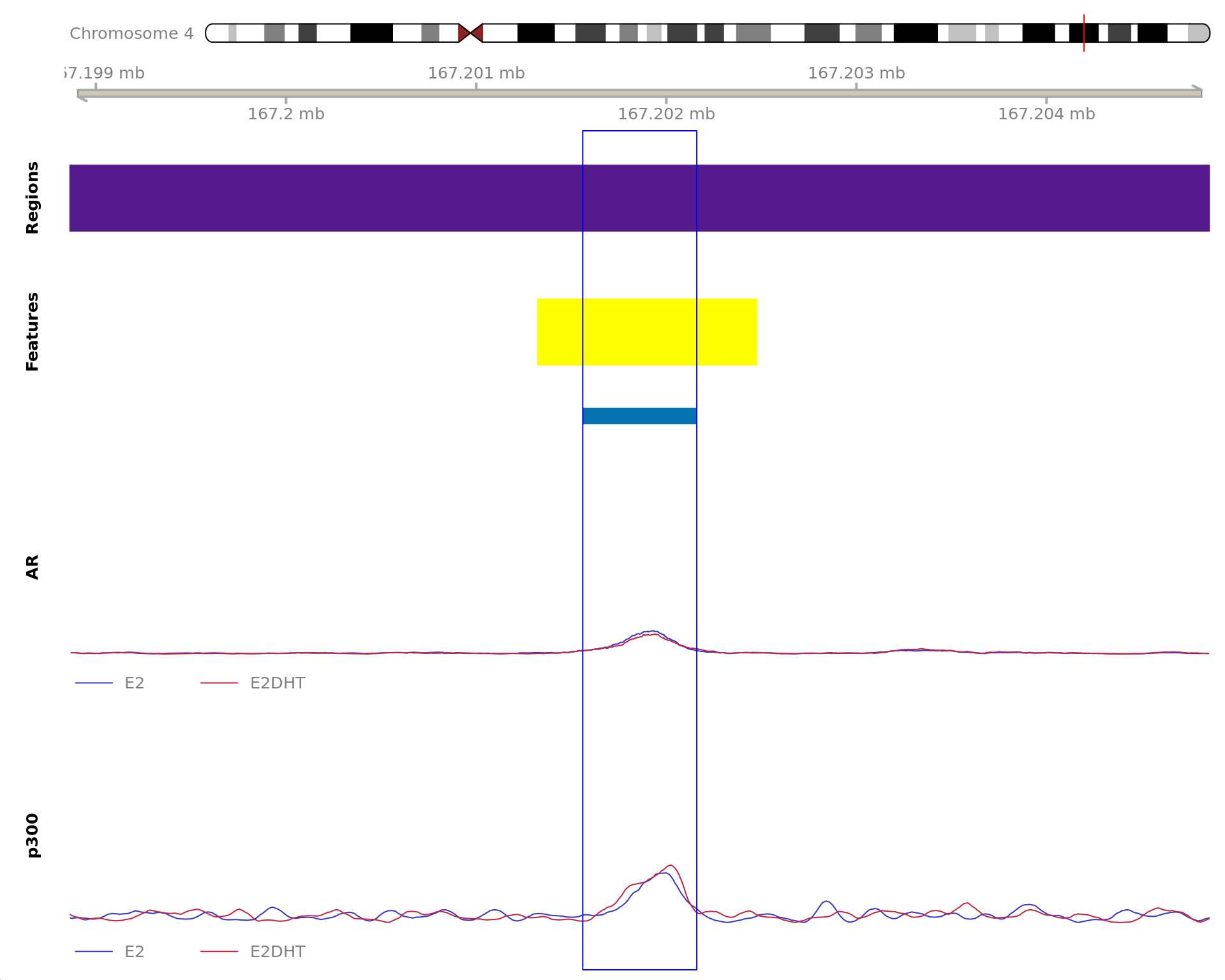
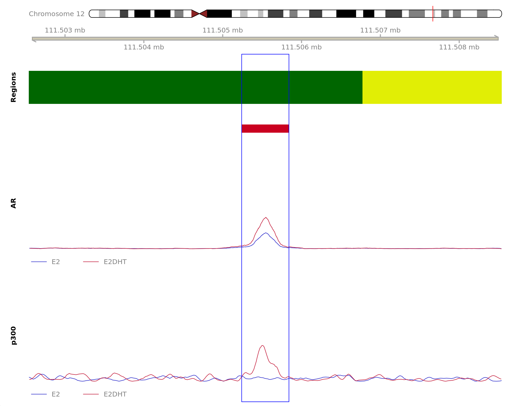
The 880bp region showing increased AR binding in response to E2DHT
treatment (FDR = 0.001). The range mostly overlapped with an Intergenic
(<10kb) region, with all defined regions shown as a contiguous bar.
Using the features supplied in enhancer_atlas_2.0_zr75.gtf.gz, this
mostly overlapped an Enhancer, shown as a separate block with the
gene-centric regions. A union peak overlapping this region was
identified by macs2 callpeak when using merged samples.
Using the above mapping strategy, this range is likely to regulate
DTX3L, HSPBAP1, PARP9 and PARP14 For each sample, the y-axis limits
represent the values from the window with the highest signal.
The 1200bp region showing increased AR binding in response to E2DHT
treatment (FDR = 1.08e-12). The range mostly overlapped with an Intron,
with all defined regions shown as a contiguous bar. Using the features
supplied in enhancer_atlas_2.0_zr75.gtf.gz, this mostly overlapped an
Enhancer, shown as a separate block with the gene-centric regions. A
union peak overlapping this region was identified by
macs2 callpeak when using merged samples. Using the above
mapping strategy, this range is likely to regulate CEP128 For each
sample, the y-axis limits represent the values from the window with the
highest signal.
The 600bp region showing increased AR binding in response to E2DHT
treatment (FDR = 3.82e-11). The range mostly overlapped with an Intron,
with all defined regions shown as a contiguous bar. Using the features
supplied in enhancer_atlas_2.0_zr75.gtf.gz, this mostly overlapped a No
Feature, shown as a separate block with the gene-centric regions. A
union peak overlapping this region was identified by
macs2 callpeak when using merged samples. No genes were
able to be assigned to this region. For each sample, the y-axis limits
represent the values from the window with the highest signal.
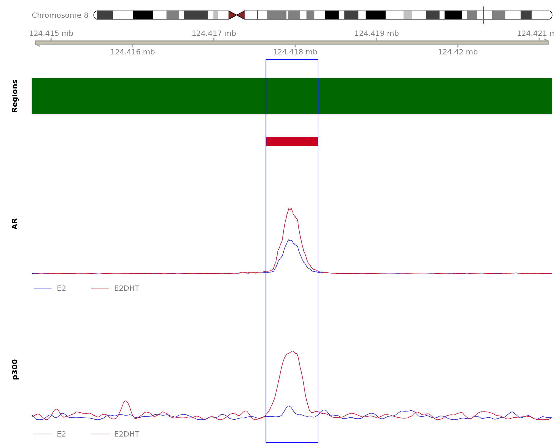
The 640bp region showing increased AR binding in response to E2DHT
treatment (FDR = 4.37e-12). The range mostly overlapped with an Intron,
with all defined regions shown as a contiguous bar. Using the features
supplied in enhancer_atlas_2.0_zr75.gtf.gz, this mostly overlapped a No
Feature, shown as a separate block with the gene-centric regions. No
union peak was identified using macs2 callpeak. Using the
above mapping strategy, this range is likely to regulate ATAD2 For each
sample, the y-axis limits represent the values from the window with the
highest signal.
As an initial exploration, the retained windows were compared to
pre-defined gene-sets. These were taken from the MSigDB
database and the gene-sets used for enrichment testing were restricted
to only include those with between 5 and 1000 genes.
Retained windows were tested for enrichment of these gene-sets
using:
Any window mapped to a gene from these gene-sets
Any window with evidence of differential binding mapped to a gene
from these gene-sets
In the first case, mapped genes were tested for enrichment against
all annotated genes, or all detected genes if RNA-Seq data was provided.
In the second case, i.e. Differentially Bound Windows, the control set
of genes were those mapped to a window (i.e. those test set from step
1). All adjusted p-values below are calculated using the
Benjamini-Hochberg FDR adjustment. After adjustment, any enriched
gene-sets with fewer than 3 mapped genes were excluded as being
uninformative.
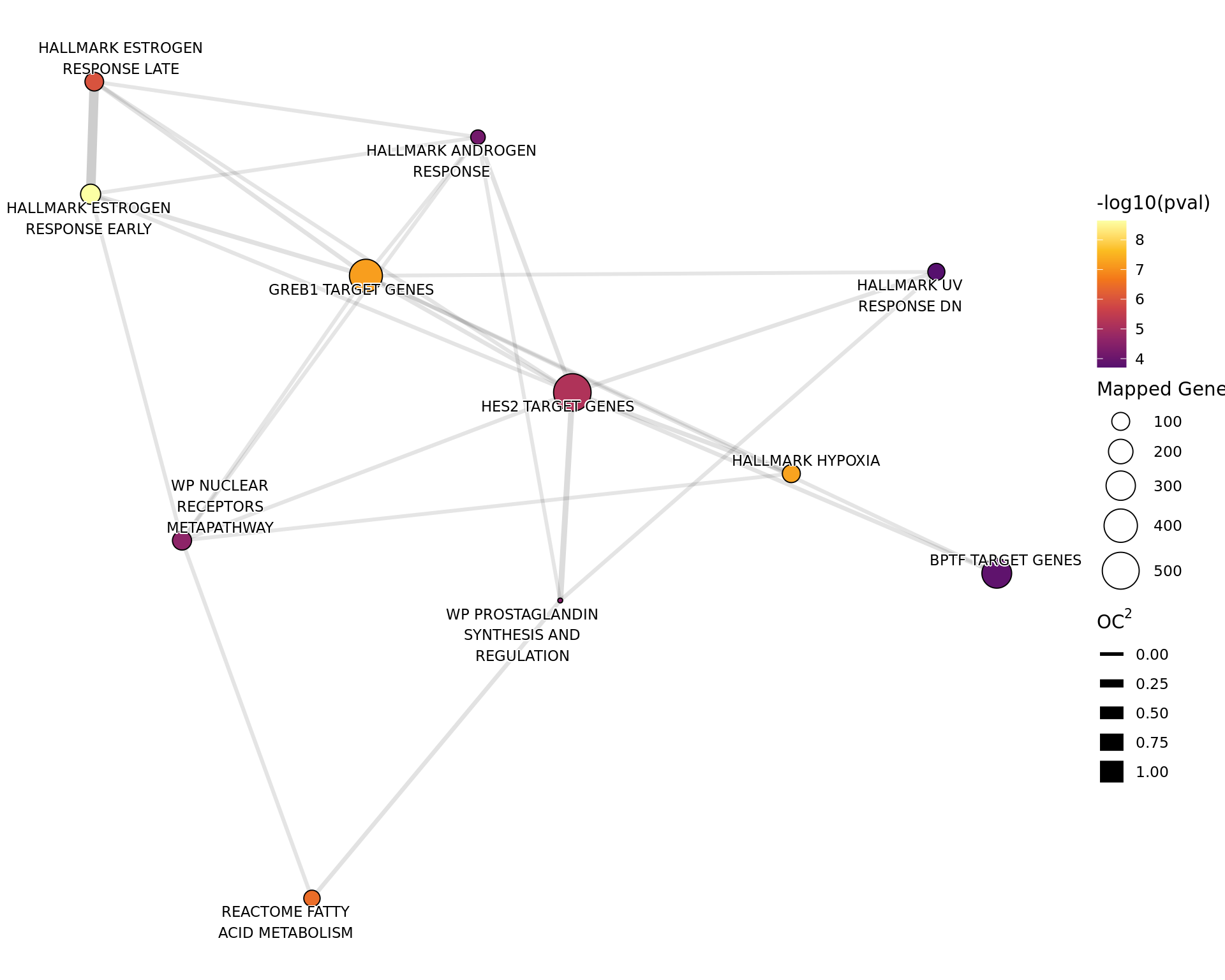
If 4 or more gene-sets were considered to be enriched, a network plot
will be produced for that specific analysis, with network sizes capped
at 80. The distances between gene-sets were calculated using the overlap
coefficient (OC). Gene-sets with a large overlap will thus be given
small distances and in the case of a complete overlap (\(OC = 1\)) the only most highly ranked
gene-set was retained. Gene-set (i.e. node) pairs with a distance >
0.9 will not have edges drawn between them and edge width also
corresponds to the distance between nodes with closely related nodes
having thicker edges. All network plots were generated using the fr
layout algorithm.
All 11 gene sets considered as
significantly enriched (p
adj < 0.05) amongst the merged windows with detectable AR
binding. Genes mapped to a merged window were compared to those not
mapped to any merged windows. Gene width was used to capture any
gene-level sampling bias.
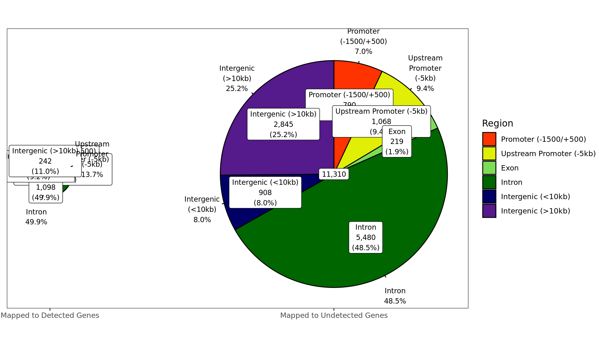
The distribution of merged windows, where AR was considered as
present, was firstly compared to genes within the RNA-Seq dataset. Genes
were simply considered as detected if present in the RNA-Seq data, or
undetected if not present. Gene-centric regions were as defined
previously.
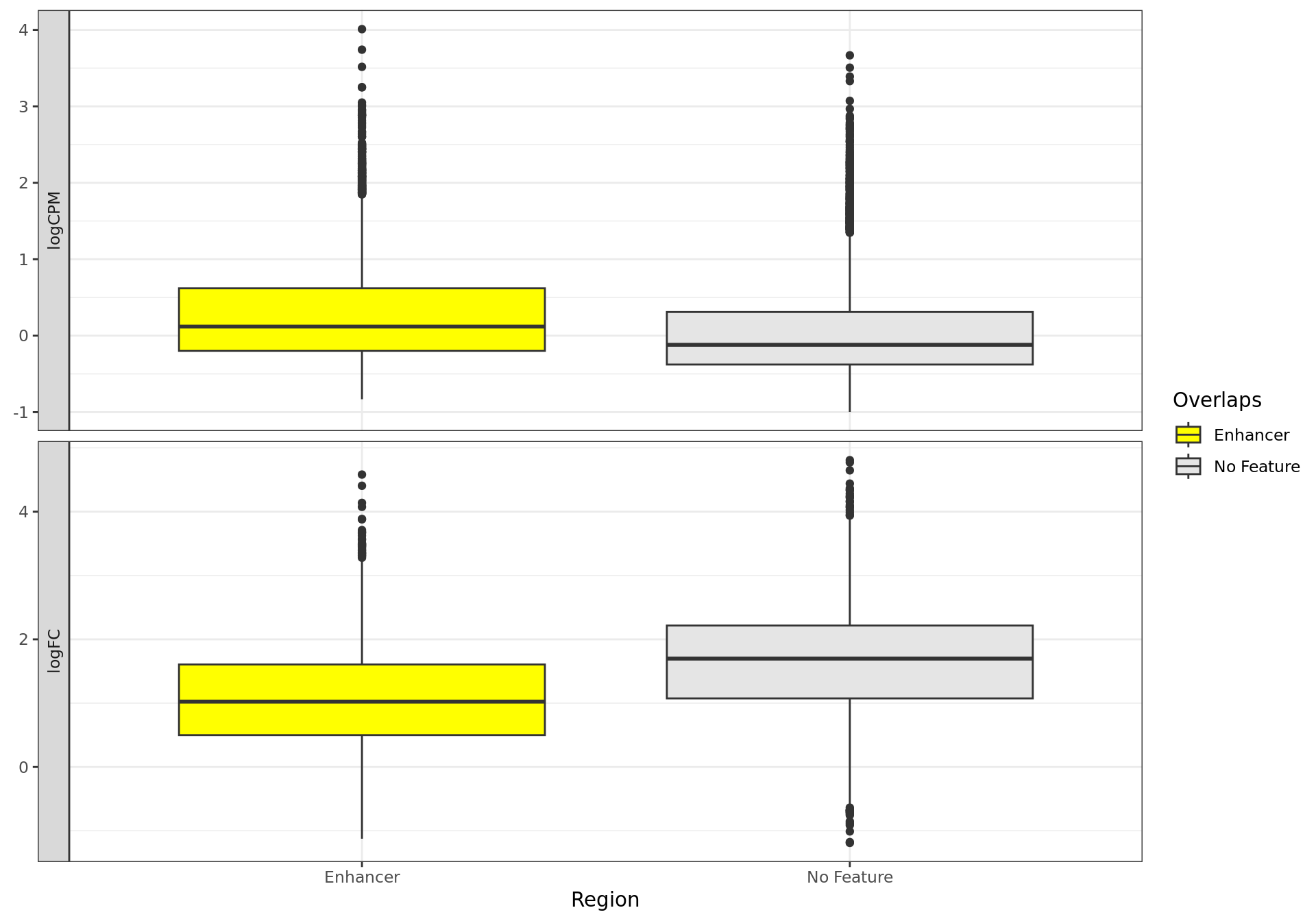
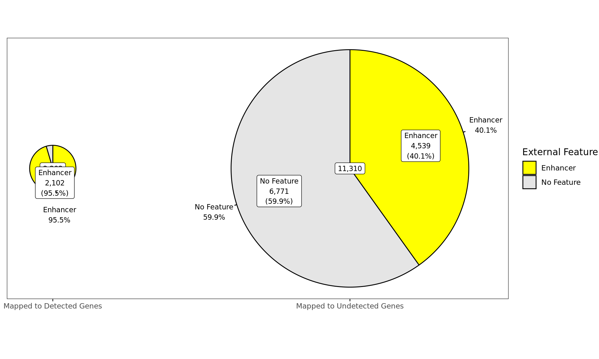
Distribution of AR-bound windows by externally-defined features from
enhancer_atlas_2.0_zr75.gtf.gz, according to whether the window is
mapped to a detected gene in the RNA-Seq dataset.
de_genes_db_regions <- tibble()
any_diff_sites <- sum(mcols(merged_results)[[fdr_column]] < fdr_alpha) > 0
any_de <- any(rnaseq$DE)
para <- ""
if (any_de & any_diff_sites) {
  ft_data <- rnaseq %>%
    dplyr::filter(gene_id %in% unlist(diff_windows)) %>%
    mutate(
      window = case_when(
        gene_id %in% unlist(diff_windows[c("Up", "Down")]) ~ "Diff",
        TRUE ~ "Unchanged"
      ) %>%
        fct_infreq()
    ) %>%
    group_by(DE, window) %>%
    tally() %>%
    pivot_wider(
      names_from = "DE", values_from = "n",
      names_prefix = "DE_", values_fill = 0
    ) %>%
    as.data.frame() %>%
    column_to_rownames("window") %>%
    as.matrix()
  ft <- fisher.test(ft_data)
  para <- glue(
    "
    Using the {comma(length(unique(unlist(diff_windows))))} genes mapped to a
    {target} binding site, genes were tested for any association between sites
    showing evidence of diferential binding and differential expression.
    {comma(length(unique(unlist(diff_windows[c('Up', 'Down')]))))} genes were
    mapped to at least one site showing differential {target} binding with
    {comma(ft_data['Diff', 'DE_TRUE'])}
    ({percent(ft_data['Diff', 'DE_TRUE'] / sum(ft_data['Diff',]))}) of these
    being considered differentially expressed. This compares to
    {percent(ft_data['Unchanged', 'DE_TRUE'] / sum(ft_data['Unchanged', ]), 0.1)}
    of genes where no differential {target} binding was detected. Fisher's
    Exact test for any association gave this a p-value of
    {ifelse(ft$p.value < 0.01, sprintf('%.2e', ft$p.value), round(ft$p.value, 3))}.
    "
  )
}
Using the 6,034 genes mapped to a AR binding site, genes were tested
for any association between sites showing evidence of diferential
binding and differential expression. 5,001 genes were mapped to at least
one site showing differential AR binding with 97 (2%) of these being
considered differentially expressed. This compares to 0.5% of genes
where no differential AR binding was detected. Fisher’s Exact test for
any association gave this a p-value of 2.92e-04.
range_js <- JS(
  "function(values) {
    var min_val = Math.round(100 * Math.min(...values)) / 100
    var max_val = Math.round(100 * Math.max(...values)) / 100
    if (min_val == max_val) {
      var ret_val = min_val.toString()
    } else {
      var ret_val = '[' + min_val.toString() + ', ' + max_val.toString() + ']'
    }
    return ret_val
  }"
)
max_signal <- max(merged_results$AveExpr)
feat_def <- NULL
if (has_features) feat_def = list(
  feature = colDef (
    name = "Feature",
    aggregate = "unique"
  )
)
cp <-  htmltools::em(
  glue(
    "
    Differentially Expressed (DE) genes were checked for {target} binding
    regions which showed evidence of changed binding.
    {comma(length(unique(de_genes_db_regions$range)), 1)} unique regions were
    mapped to {comma(length(unique(de_genes_db_regions$gene_id)), 1)} DE genes.
    Data are presented in a gene-centric manner and ranges may map to multiple
    genes. The full set of ranges considered to be showing evidence of altered
    {target} binding are shown for each gene. The summarised range containing
    all mapped ranges is given in the collapsed row, along with the range of
    distances to gene and the range of signal levels. In the collapsed row, the
    value for logFC represents the average across all mapped regions, with the
    maximum FDR also shown. If {target} binding occurs within another gene this
    is indicated in the 'Region' column.
    All sites and genes were exported as {basename(all_out$de_genes)}.
    "
  )
)
fs <- 12
tbl <- de_genes_db_regions %>%
  reactable(
    groupBy = "gene_name",
    filterable = TRUE,
    borderless = TRUE,
    showPageSizeOptions = TRUE,
    columns = c(
      list(
        gene_name = colDef(
          name = "Gene", maxWidth = fs*11,
          style = list(
            borderRight = "1px solid rgba(0, 0, 0, 0.1)",
            fontSize = fs
          )
        ),
        gene_id = colDef(
          name = "ID", aggregate = "unique", cell = function(value) "",
          show = FALSE
        ),
        RNA_logFC = colDef(
          name = "logFC",
          aggregate = "mean",
          style = JS(
            glue(
            "function(rowInfo) {
              var value = rowInfo.row['RNA_logFC']
              if (value < 0) {
                var color = '{{direction_colours[['Down']]}}'
              } else if (value > 0) {
                var color = '{{direction_colours[['Up']]}}'
              } else {
                var color = '#000000'
              }
              return { color: color, fontSize: {{fs}} }
            }",
            .open = "{{", .close = "}}"
            )
          ),
          format = colFormat(digits= 2),
          maxWidth = fs*6,
          cell = function(value) ""
        ),
        RNA_FDR = colDef(
          name = "FDR",
          aggregate = "min",
          format = colFormat(digits = 4),
          maxWidth = fs*6,
          cell = function(value) "",
          style = list(
            borderRight = "1px solid rgba(0, 0, 0, 0.1)",
            fontSize = fs
          )
        ),
        range = colDef(
          name = "Range",
          minWidth = 160,
          aggregate = JS(
            "function(values){
              var chrom = [];
              var rng = [];
              var start = [];
              var end = [];
              for (i = 0; i < values.length; i++) {
                chrom[i] = values[i].split(':')[0];
                rng[i] = values[i].split(':')[1];
                start[i] = rng[i].split('-')[0];
                end[i] = rng[i].split('-')[1];
              }

              min_start = Math.min(...start);
              max_end = Math.max(...end);
              var ret_val = [...new Set(chrom)] + ':' + min_start.toString() + '-' + max_end.toString();

              return ret_val

            }"
          )
        ),
        dist2Gene = colDef(
          name = "Distance to Gene",
          aggregate = range_js,
          format = colFormat(digits = 0, separators = TRUE),
          maxWidth = fs*8,
          style = list(
            borderRight = "1px solid rgba(0, 0, 0, 0.1)",
            fontSize = fs
          ),
        ),
        ChIP_logCPM = colDef(
          name = "logCPM",
          maxWidth = fs*6,
          aggregate = range_js,
          format = colFormat(digits = 2),
          style = function(value) bar_style(
            width = value / max_signal, fontSize = fs
          )
        ),
        ChIP_logFC = colDef(
          name = "logFC",
          aggregate = "mean",
          maxWidth = fs*5,
          format = colFormat(digits = 2),
          cell = function(value) sprintf("%.2f", value),
          style =  JS(
            glue(
            "function(rowInfo) {
              var value = rowInfo.row['ChIP_logFC']
              if (value < 0) {
                var color = '{{direction_colours[['Down']]}}'
              } else if (value > 0) {
                var color = '{{direction_colours[['Up']]}}'
              } else {
                var color = '#000000'
              }
              return { color: color, fontSize: {{fs}} }
            }",
            .open = "{{", .close = "}}"
            )
          )
        ),
        ChIP_FDR = colDef(
          name = "FDR",
          aggregate = "max",
          maxWidth = 10 + fs*5,
          format = colFormat(prefix = "< ", digits = 4),
          cell = function(value) ifelse(
            value < 0.001,
            sprintf("%.2e", value),
            sprintf("%.3f", value)
          )
        ),
        overlaps_ref = colDef(
          name = "Macs Peak",
          show = FALSE,
          aggregate = "frequency",
          cell = function(value) ifelse(value, "\u2714 Yes", "\u2716 No"),
          style = function(value) {
            color <- ifelse(value, "#008000", "#e00000")
            list(color = color, fontSize = fs)
          },
          maxWidth = fs*5
        ),
        status = colDef(
          name = "Status",
          aggregate = "frequency",
          maxWidth = fs*6,
          cell = function(value) {
            html_symbol <- ""
            if (str_detect(value, "Up")) html_symbol <- "\u21E7"
            if (str_detect(value, "Down")) html_symbol <- "\u21E9"
            paste(html_symbol, value)
          },
          style = JS(
            glue(
            "function(rowInfo) {
              var value = rowInfo.row['ChIP_logFC']
              if (value < 0) {
                var color = '{{direction_colours[['Down']]}}'
              } else if (value > 0) {
                var color = '{{direction_colours[['Up']]}}'
              } else {
                var color = '#000000'
              }
              return { color: color, fontSize: {{fs}} }
            }",
            .open = "{{", .close = "}}"
            )
          )
        ),
        region = colDef(
          name = "Binding Region",
          aggregate = "unique"
        )
      ),
      feat_def
    ),
    columnGroups = list(
      colGroup(name = "RNA-Seq", columns = c("RNA_logFC", "RNA_FDR")),
      colGroup(
        name = paste(target, "ChIP-Seq"),
        columns = c("ChIP_logCPM", "ChIP_logFC", "ChIP_FDR", "status")
      )
    ),
    theme = reactableTheme(style = list(fontSize = fs))
  )
div(class = "table",
  div(class = "table-header",
      div(class = "caption", cp),
      tbl
  )
)
Differentially Expressed (DE) genes were checked for AR binding
regions which showed evidence of changed binding.
298 unique regions were
mapped to 97 DE genes.
Data are presented in a gene-centric manner and ranges may map to multiple
genes. The full set of ranges considered to be showing evidence of altered
AR binding are shown for each gene. The summarised range containing
all mapped ranges is given in the collapsed row, along with the range of
distances to gene and the range of signal levels. In the collapsed row, the
value for logFC represents the average across all mapped regions, with the
maximum FDR also shown. If AR binding occurs within another gene this
is indicated in the 'Region' column.
All sites and genes were exported as AR_E2_E2DHT-DE_genes.csv.
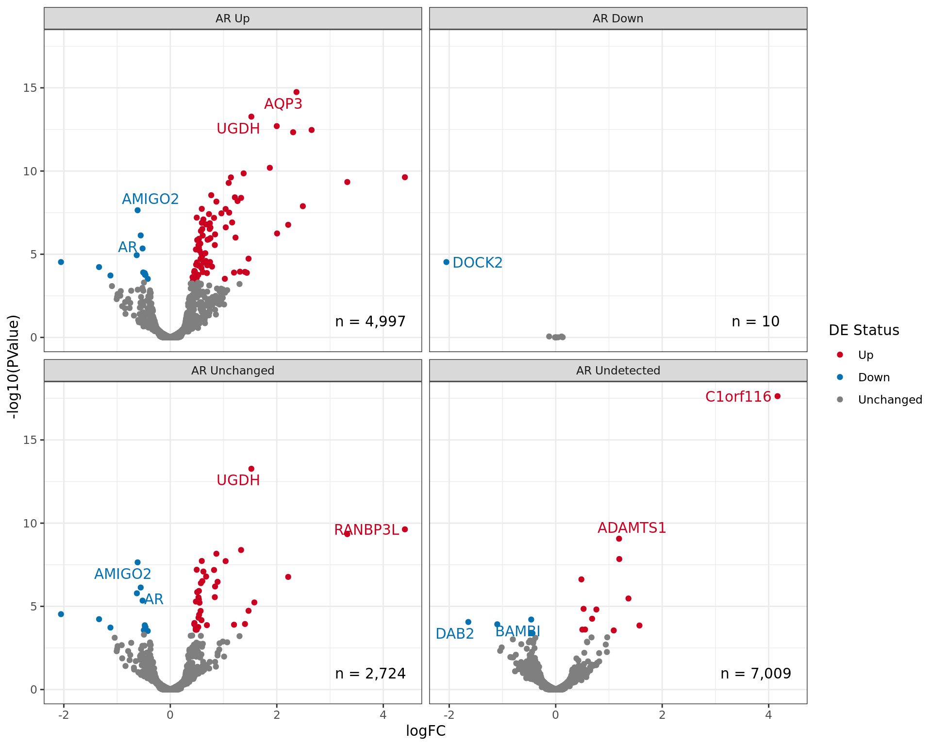
Volcano plot showing gene expression patterns separated by AR
status. The two most highly ranked genes for up and down regulation are
labelled in each panel. Given that some genes may be mapped to multiple
AR binding events which include different binding patterns, genes may
appear in multiple panels.
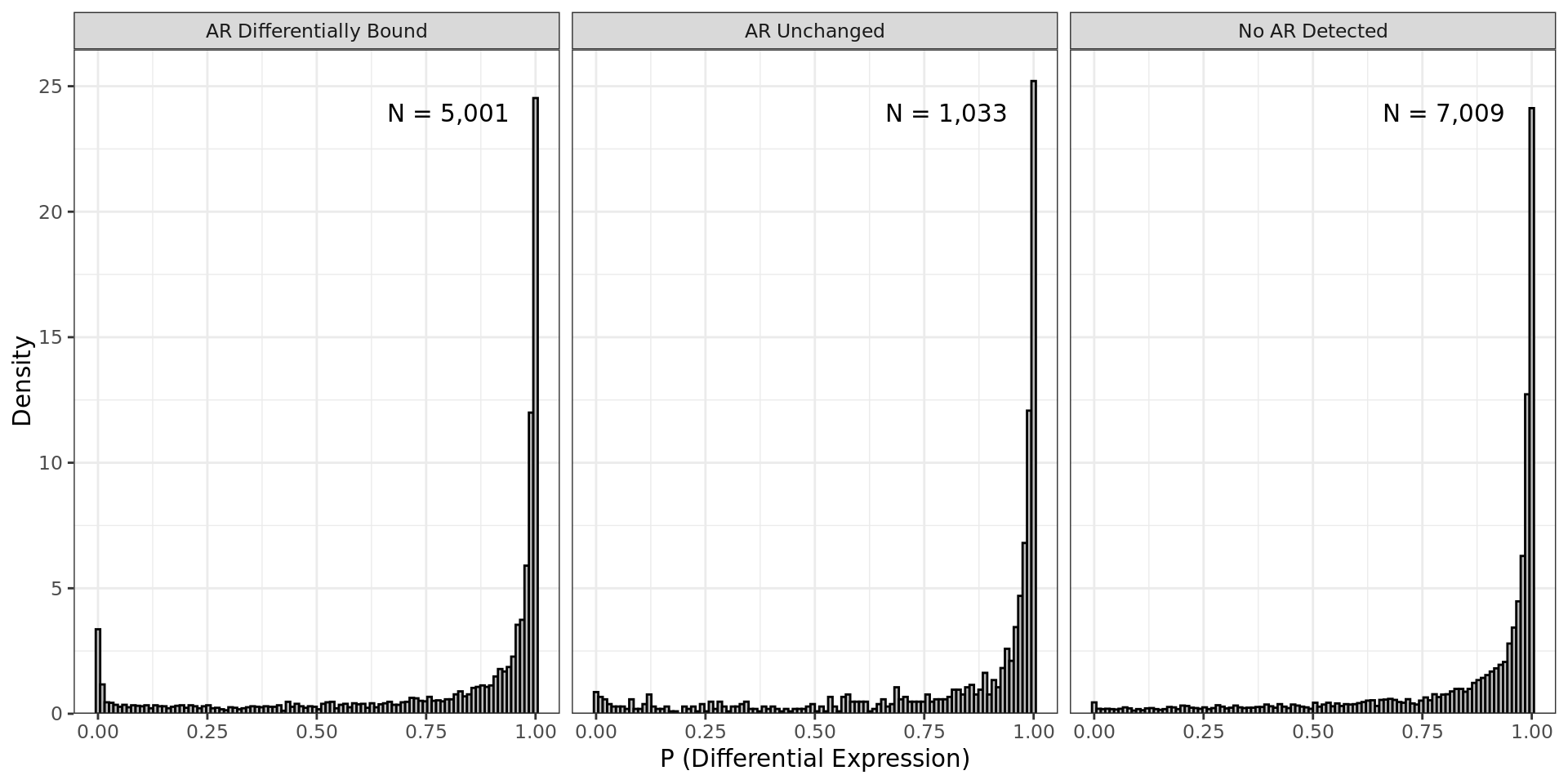
P-Values for differential expression partitioned by AR ChIP peak
status. Genes were considered as being mapped to a differentially bound
peak if one or more peaks was considered as differentially bound. No IHW
procedure was undertaken using this data.
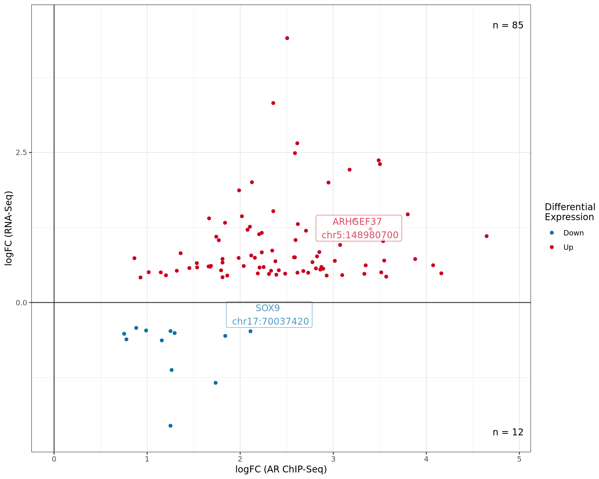
logFC values for differentially bound ChIP-Seq peaks mapped to DE
genes. The most highly ranked peak for each quandrant is labelled at
showing both the gene and centre of the binding region. Whilst binding
sites may be mapped to multiple genes, only the most highly ranked
binding site is shown mapped to the mosthighly ranked DE genes. Points
are coloured by differential expression status.
Binding Pattern GSEA
GSEA By Direction of Regulation
GSEA analysis was first performed by taking the genes mapped to
various sets of peaks, and checking for enrichment amongst the RNA-Seq
results, ranking genes from up- to down-regulated, by significance of
the logFC estimates.
cp <-  htmltools::em(
  glue(
    "Merged windows were mapped to genes and their position amongst the ",
    "RNA-Seq results was assessed. Windows were classified based on  ",
    "the direction of {target} binding with ",
    "{treat_levels[[2]]} treatment. {nrow(gsea_dir_sig)} sets of windows were ",
    "associated with changes in gene expression, using the sign of ",
    "fold-change and ranking statistic to initially rank the ",
    "{comma(nrow(rnaseq), 1)} genes considered as detected."
  )
)
tbl <- gsea_dir_sig %>%
  mutate(
    `Edge Size` = vapply(leadingEdge, length, integer(1)),
    leadingEdge = lapply(leadingEdge, function(x) id2gene[x]) %>%
      vapply(paste, character(1), collapse = "; "),
    Direction = ifelse(NES > 0, "\u21E7 Up-regulated", "\u21E9 Down-regulated"),
    "{target}" := str_extract(pathway, "(Up|Down|Unchanged)$"),
    pathway = str_remove_all(pathway, " / [^/]+$")
  ) %>%
  dplyr::select(
    !!sym(target), Windows = size, Direction,
    p = pval, padj, `Edge Size`, `Leading Edge` = leadingEdge
  ) %>%
  reactable(
    filterable = TRUE,
    columns = list2(
      "{target}" := colDef(
        maxWidth = 90,
        cell = function(value) {
          html_symbol <- ""
          if (str_detect(value, "Up")) html_symbol <- "\u21E7"
          if (str_detect(value, "Down")) html_symbol <- "\u21E9"
          paste(html_symbol, value)
        },
        style = function(value) {
          colour <- case_when(
            str_detect(value, "Up") ~ colours$direction[["up"]],
            str_detect(value, "Down") ~ colours$direction[["down"]],
            TRUE ~ colours$direction[["unchanged"]]
          )
          list(color = colour)
        }
      ),
      Windows = colDef(maxWidth = 80, format = colFormat(separators = TRUE)),
      Direction = colDef(
        name = "Gene Direction",
        maxWidth = 150,
        style = function(value) {
          colour <- ifelse(
            str_detect(value, "Up"),
            colours$direction[["up"]],
            colours$direction[["down"]]
          )
          list(color = colour)
        },
      ),
      p = colDef(
        cell = function(value) sprintf("%.2e", value), maxWidth = 80
      ),
      padj = colDef(
        name = glue("p<sub>{adj_method}</sub>"), html = TRUE,
        cell = function(value) {
          ifelse(
            value < 0.001, sprintf("%.2e", value), sprintf("%.3f", value)
          )
        }
      ),
      "Edge Size" = colDef(maxWidth = 80),
     "Leading Edge" = colDef(
       minWidth = 150,
       cell = function(value) with_tooltip(value, width = 50)
     )
    )
  )
div(class = "table",
  div(class = "table-header",
      div(class = "caption", cp),
      tbl
  )
)
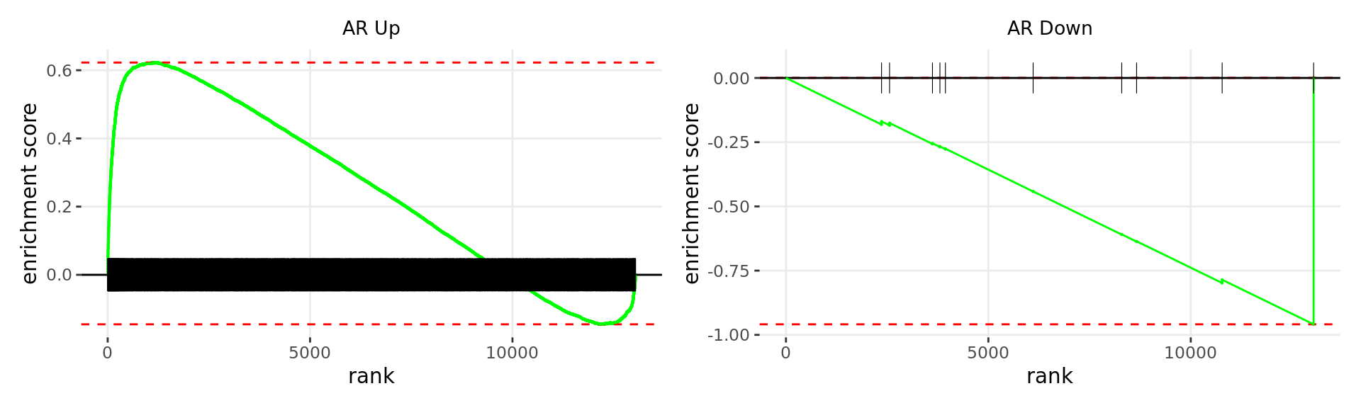
Merged windows were mapped to genes and their position amongst the RNA-Seq results was assessed. Windows were classified based on the direction of AR binding with E2DHT treatment. 2 sets of windows were associated with changes in gene expression, using the sign of fold-change and ranking statistic to initially rank the 13,043 genes considered as detected.
wrap_plots(p)
Barcode plots for the top 2 sets of windows associated with
directional changes in gene expression.
cp <-  htmltools::em(
  glue(
    "Merged windows were mapped to genes and their position amongst the ",
    "RNA-Seq results was assessed. Windows were classified based on which ",
    "region was the best overlap, and the direction of {target} binding with ",
    "{treat_levels[[2]]} treatment. {nrow(gsea_reg_dir_sig)} sets of windows were ",
    "associated with changes in gene expression, using the sign of ",
    "fold-change and ranking statistic to initially rank the ",
    "{comma(nrow(rnaseq), 1)} genes considered as detected."
  )
)
tbl <- gsea_reg_dir_sig %>%
  mutate(
    `Edge Size` = vapply(leadingEdge, length, integer(1)),
    leadingEdge = lapply(leadingEdge, function(x) id2gene[x]) %>%
      vapply(paste, character(1), collapse = "; "),
    Direction = ifelse(NES > 0, "\u21E7 Up-regulated", "\u21E9 Down-regulated"),
    "{target}" := str_extract(pathway, "(Up|Down|Unchanged)$"),
    pathway = str_remove_all(pathway, " / [^/]+$")
  ) %>%
  dplyr::select(
    pathway, !!sym(target), Windows = size, Direction,
    p = pval, padj, `Edge Size`, `Leading Edge` = leadingEdge
  ) %>%
  reactable(
    filterable = TRUE,
    columns = list2(
      pathway = colDef(
        minWidth = 100, name = "Region"
      ),
      "{target}" := colDef(
        maxWidth = 90,
        cell = function(value) {
          html_symbol <- ""
          if (str_detect(value, "Up")) html_symbol <- "\u21E7"
          if (str_detect(value, "Down")) html_symbol <- "\u21E9"
          paste(html_symbol, value)
        },
        style = function(value) {
          colour <- case_when(
            str_detect(value, "Up") ~ colours$direction[["up"]],
            str_detect(value, "Down") ~ colours$direction[["down"]],
            TRUE ~ colours$direction[["unchanged"]]
          )
          list(color = colour)
        }
      ),
      Windows = colDef(maxWidth = 80, format = colFormat(separators = TRUE)),
      Direction = colDef(
        name = "Gene Direction",
        maxWidth = 150,
        style = function(value) {
          colour <- ifelse(
            str_detect(value, "Up"),
            colours$direction[["up"]],
            colours$direction[["down"]]
          )
          list(color = colour)
        },
      ),
      p = colDef(
        cell = function(value) sprintf("%.2e", value), maxWidth = 80
      ),
      padj = colDef(
        name = glue("p<sub>{adj_method}</sub>"), html = TRUE,
        cell = function(value) {
          ifelse(
            value < 0.001, sprintf("%.2e", value), sprintf("%.3f", value)
          )
        }
      ),
      "Edge Size" = colDef(maxWidth = 80),
     "Leading Edge" = colDef(
       minWidth = 150,
       cell = function(value) with_tooltip(value, width = 50)
     )
    )
  )
div(class = "table",
  div(class = "table-header",
      div(class = "caption", cp),
      tbl
  )
)
Merged windows were mapped to genes and their position amongst the RNA-Seq results was assessed. Windows were classified based on which region was the best overlap, and the direction of AR binding with E2DHT treatment. 7 sets of windows were associated with changes in gene expression, using the sign of fold-change and ranking statistic to initially rank the 13,043 genes considered as detected.
wrap_plots(p)
Barcode plots for the top 7 sets of windows associated with
directional changes in gene expression.
cp <-  htmltools::em(
  glue(
    "Merged windows were mapped to genes and their position amongst the ",
    "RNA-Seq results was assessed. Windows were classified based on which ",
    "feature was the best overlap, and the direction of {target} binding with ",
    "{treat_levels[[2]]} treatment. {nrow(gsea_feat_dir_sig)} sets of windows were ",
    "associated with changes in gene expression, using the sign of ",
    "fold-change and ranking statistic to initially rank the ",
    "{comma(nrow(rnaseq), 1)} genes considered as detected."
  )
)
tbl <- gsea_feat_dir_sig %>%
  mutate(
    `Edge Size` = vapply(leadingEdge, length, integer(1)),
    leadingEdge = lapply(leadingEdge, function(x) id2gene[x]) %>%
      vapply(paste, character(1), collapse = "; "),
    Direction = ifelse(NES > 0, "\u21E7 Up-regulated", "\u21E9 Down-regulated"),
    "{target}" := str_extract(pathway, "(Up|Down|Unchanged)$"),
    pathway = str_remove_all(pathway, " / [^/]+$")
  ) %>%
  dplyr::select(
    pathway, !!sym(target), Windows = size, Direction,
    p = pval, FDR = padj, `Edge Size`, `Leading Edge` = leadingEdge
  ) %>%
  reactable(
    filterable = TRUE,
    columns = list2(
      pathway = colDef(
        minWidth = 100, name = "Region"
      ),
      "{target}" := colDef(
        maxWidth = 120,
        cell = function(value) {
          html_symbol <- ""
          if (str_detect(value, "Up")) html_symbol <- "\u21E7"
          if (str_detect(value, "Down")) html_symbol <- "\u21E9"
          paste(html_symbol, value)
        },
        style = function(value) {
          colour <- case_when(
            str_detect(value, "Up") ~ colours$direction[["up"]],
            str_detect(value, "Down") ~ colours$direction[["down"]],
            TRUE ~ colours$direction[["unchanged"]]
          )
          list(color = colour)
        }
      ),
      Windows = colDef(maxWidth = 80, format = colFormat(separators = TRUE)),
      Direction = colDef(
        name = "Gene Direction",
        maxWidth = 120,
        style = function(value) {
          colour <- ifelse(
            str_detect(value, "Up"),
            colours$direction[["up"]],
            colours$direction[["down"]]
          )
          list(color = colour)
        },
      ),
      p = colDef(
        cell = function(value) sprintf("%.2e", value), maxWidth = 80
      ),
      FDR = colDef(
        cell = function(value) sprintf("%.2e", value), maxWidth = 80
      ),
      "Edge Size" = colDef(maxWidth = 80),
     "Leading Edge" = colDef(
       minWidth = 150,
       cell = function(value) with_tooltip(value, width = 50)
     )
    )
  )
div(class = "table",
  div(class = "table-header",
      div(class = "caption", cp),
      tbl
  )
)
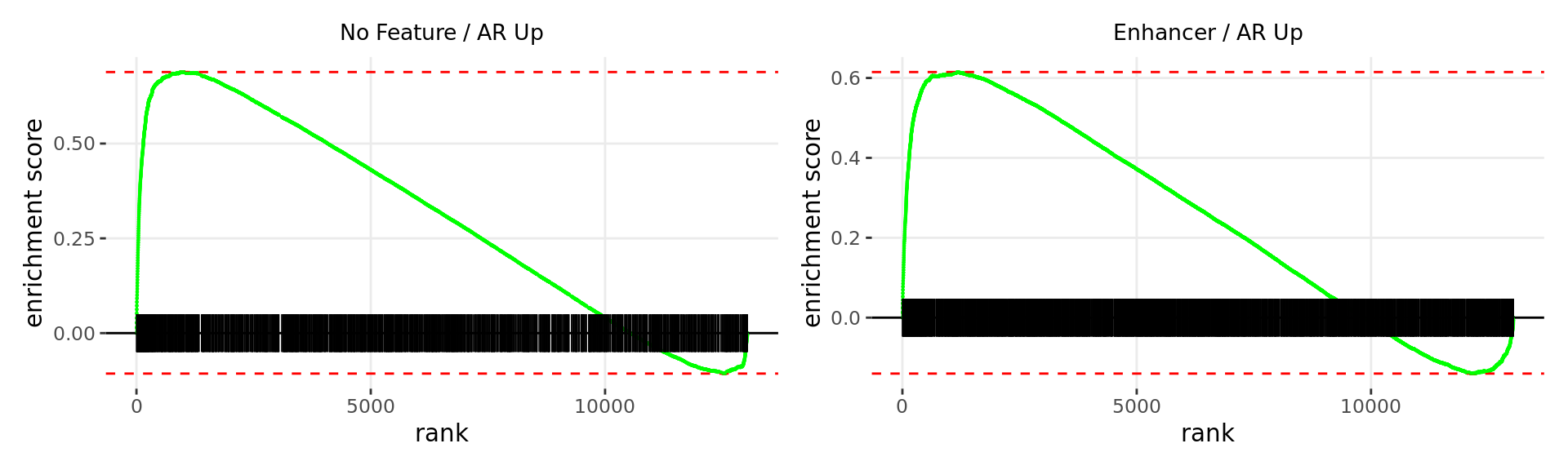
Merged windows were mapped to genes and their position amongst the RNA-Seq results was assessed. Windows were classified based on which feature was the best overlap, and the direction of AR binding with E2DHT treatment. 2 sets of windows were associated with changes in gene expression, using the sign of fold-change and ranking statistic to initially rank the 13,043 genes considered as detected.
wrap_plots(p)
Barcode plots for the top 2 sets of windows associated with
directional changes in gene expression.
GSEA By Significance Only
GSEA analysis was then performed by taking the genes mapped to
various sets of peaks, and checking for enrichment amongst the RNA-Seq
results, ranking genes only from least to most significant, which
effectively treats up- and down-regulation as indistinguishable.
cp <-  htmltools::em(
  glue(
    "Merged windows were mapped to genes and their position amongst the ",
    "RNA-Seq results was assessed. Windows were classified based on  ",
    "the direction of {target} binding with ",
    "{treat_levels[[2]]} treatment. {nrow(gsea_nondir_sig)} sets of windows were ",
    "associated with changes in gene expression, using only the p-value to ",
    "rank the {comma(nrow(rnaseq), 1)} genes considered as detected."
  )
)
tbl <- gsea_nondir_sig %>%
  mutate(
    `Edge Size` = vapply(leadingEdge, length, integer(1)),
    leadingEdge = lapply(leadingEdge, function(x) id2gene[x]) %>%
      vapply(paste, character(1), collapse = "; "),
    "{target}" := str_extract(pathway, "(Up|Down|Unchanged)$"),
    pathway = str_remove_all(pathway, " / [^/]+$")
  ) %>%
  dplyr::select(
    !!sym(target), Windows = size, p = pval, FDR = padj,
    `Edge Size`, `Leading Edge` = leadingEdge
  ) %>%
  reactable(
    filterable = TRUE,
    columns = list2(
      "{target}" := colDef(
        maxWidth = 150,
        cell = function(value) {
          html_symbol <- ""
          if (str_detect(value, "Up")) html_symbol <- "\u21E7"
          if (str_detect(value, "Down")) html_symbol <- "\u21E9"
          paste(html_symbol, value)
        },
        style = function(value) {
           colour <- case_when(
            str_detect(value, "Up") ~ colours$direction[["up"]],
            str_detect(value, "Down") ~ colours$direction[["down"]],
            TRUE ~ colours$direction[["unchanged"]]
          )
          list(color = colour)
        }
      ),
      Windows = colDef(maxWidth = 80, format = colFormat(separators = TRUE)),
      p = colDef(
        cell = function(value) sprintf("%.2e", value), maxWidth = 80
      ),
      FDR = colDef(
        cell = function(value) sprintf("%.2e", value), maxWidth = 80
      ),
      "Edge Size" = colDef(maxWidth = 80),
     "Leading Edge" = colDef(
       minWidth = 150,
       cell = function(value) with_tooltip(value, width = 50)
     )
    )
  )
div(class = "table",
  div(class = "table-header",
      div(class = "caption", cp),
      tbl
  )
)
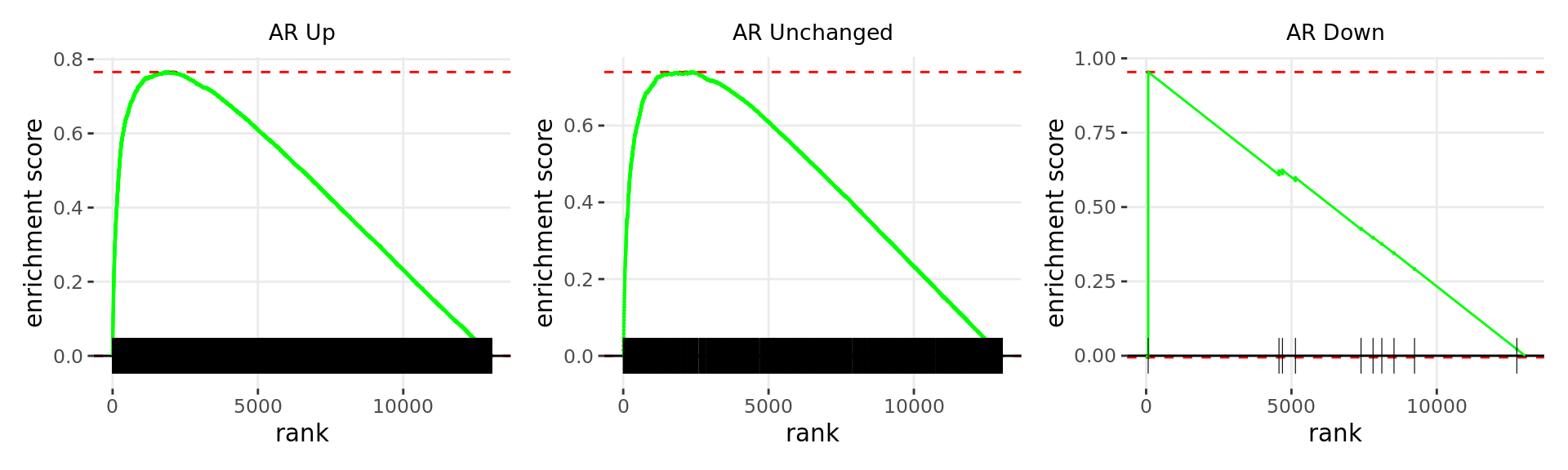
Merged windows were mapped to genes and their position amongst the RNA-Seq results was assessed. Windows were classified based on the direction of AR binding with E2DHT treatment. 3 sets of windows were associated with changes in gene expression, using only the p-value to rank the 13,043 genes considered as detected.
wrap_plots(p)
Barcode plots for the top 3 sets of windows associated with
non-directional changes in gene expression.
cp <-  htmltools::em(
  glue(
    "Merged windows were mapped to genes and their position amongst the ",
    "RNA-Seq results was assessed. Windows were classified based on which ",
    "region was the best overlap, and the direction of {target} binding with ",
    "{treat_levels[[2]]} treatment. {nrow(gsea_reg_nondir_sig)} sets of windows were ",
    "associated with changes in gene expression, using only the p-value to ",
    "rank the {comma(nrow(rnaseq), 1)} genes considered as detected."
  )
)
tbl <- gsea_reg_nondir_sig %>%
  mutate(
    `Edge Size` = vapply(leadingEdge, length, integer(1)),
    leadingEdge = lapply(leadingEdge, function(x) id2gene[x]) %>%
      vapply(paste, character(1), collapse = "; "),
    "{target}" := str_extract(pathway, "(Up|Down|Unchanged)$"),
    pathway = str_remove_all(pathway, " / [^/]+$")
  ) %>%
  dplyr::select(
    pathway, !!sym(target), Windows = size, p = pval, FDR = padj,
    `Edge Size`, `Leading Edge` = leadingEdge
  ) %>%
  reactable(
    filterable = TRUE,
    columns = list2(
      pathway = colDef(
        minWidth = 100, name = "Region"
      ),
      "{target}" := colDef(
        maxWidth = 90,
        cell = function(value) {
          html_symbol <- ""
          if (str_detect(value, "Up")) html_symbol <- "\u21E7"
          if (str_detect(value, "Down")) html_symbol <- "\u21E9"
          paste(html_symbol, value)
        },
        style = function(value) {
           colour <- case_when(
            str_detect(value, "Up") ~ colours$direction[["up"]],
            str_detect(value, "Down") ~ colours$direction[["down"]],
            TRUE ~ colours$direction[["unchanged"]]
          )
          list(color = colour)
        }
      ),
      Windows = colDef(maxWidth = 80, format = colFormat(separators = TRUE)),
      p = colDef(
        cell = function(value) sprintf("%.2e", value), maxWidth = 80
      ),
      FDR = colDef(
        cell = function(value) sprintf("%.2e", value), maxWidth = 80
      ),
      "Edge Size" = colDef(maxWidth = 80),
     "Leading Edge" = colDef(
       minWidth = 150,
       cell = function(value) with_tooltip(value, width = 50)
     )
    )
  )
div(class = "table",
  div(class = "table-header",
      div(class = "caption", cp),
      tbl
  )
)
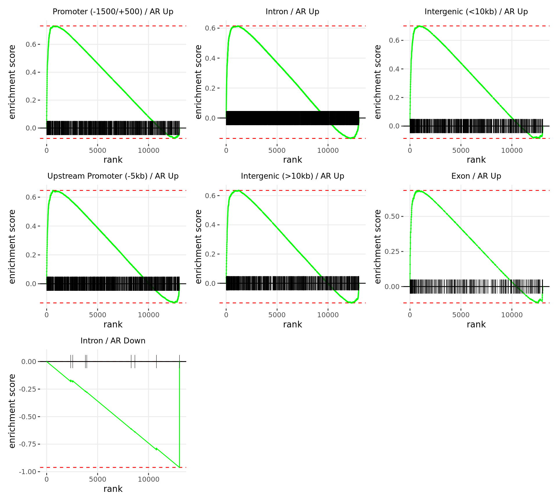
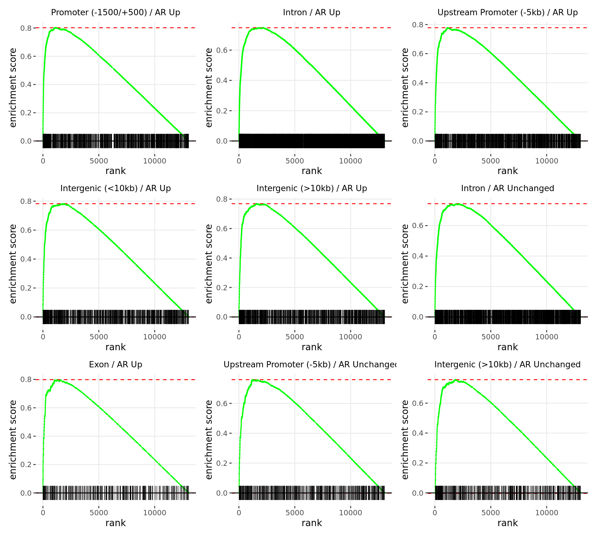
Merged windows were mapped to genes and their position amongst the RNA-Seq results was assessed. Windows were classified based on which region was the best overlap, and the direction of AR binding with E2DHT treatment. 12 sets of windows were associated with changes in gene expression, using only the p-value to rank the 13,043 genes considered as detected.
wrap_plots(p)
Barcode plots for the top 9 sets of windows associated with
non-directional changes in gene expression.
cp <-  htmltools::em(
  glue(
    "Merged windows were mapped to genes and their position amongst the ",
    "RNA-Seq results was assessed. Windows were classified based on which ",
    "feature was the best overlap, and the direction of {target} binding with ",
    "{treat_levels[[2]]} treatment. {nrow(gsea_feat_nondir_sig)} sets of windows were ",
    "associated with overall changes in gene expression, using only the ",
    "test statistic to rank the ",
    "{comma(nrow(rnaseq), 1)} genes considered as detected."
  )
)
tbl <- gsea_feat_nondir_sig %>%
  mutate(
    `Edge Size` = vapply(leadingEdge, length, integer(1)),
    leadingEdge = lapply(leadingEdge, function(x) id2gene[x]) %>%
      vapply(paste, character(1), collapse = "; "),
    Direction = ifelse(NES > 0, "\u21E7 Up-regulated", "\u21E9 Down-regulated"),
    "{target}" := str_extract(pathway, "(Up|Down|Unchanged)$"),
    pathway = str_remove_all(pathway, " / [^/]+$")
  ) %>%
  dplyr::select(
    pathway, !!sym(target), Windows = size, Direction,
    p = pval, FDR = padj, `Edge Size`, `Leading Edge` = leadingEdge
  ) %>%
  reactable(
    filterable = TRUE,
    columns = list2(
      pathway = colDef(
        minWidth = 100, name = "Region"
      ),
      "{target}" := colDef(
        maxWidth = 90,
        cell = function(value) {
          html_symbol <- ""
          if (str_detect(value, "Up")) html_symbol <- "\u21E7"
          if (str_detect(value, "Down")) html_symbol <- "\u21E9"
          paste(html_symbol, value)
        },
        style = function(value) {
          colour <- case_when(
            str_detect(value, "Up") ~ colours$direction[["up"]],
            str_detect(value, "Down") ~ colours$direction[["down"]],
            TRUE ~ colours$direction[["unchanged"]]
          )
          list(color = colour)
        }
      ),
      Windows = colDef(maxWidth = 80, format = colFormat(separators = TRUE)),
      Direction = colDef(
        name = "Gene Direction",
        maxWidth = 120,
        style = function(value) {
          colour <- ifelse(
            str_detect(value, "Up"),
            colours$direction[["up"]],
            colours$direction[["down"]]
          )
          list(color = colour)
        },
      ),
      p = colDef(
        cell = function(value) sprintf("%.2e", value), maxWidth = 80
      ),
      FDR = colDef(
        cell = function(value) sprintf("%.2e", value), maxWidth = 80
      ),
      "Edge Size" = colDef(maxWidth = 80),
     "Leading Edge" = colDef(
       minWidth = 150,
       cell = function(value) with_tooltip(value, width = 50)
     )
    )
  )
div(class = "table",
  div(class = "table-header",
      div(class = "caption", cp),
      tbl
  )
)
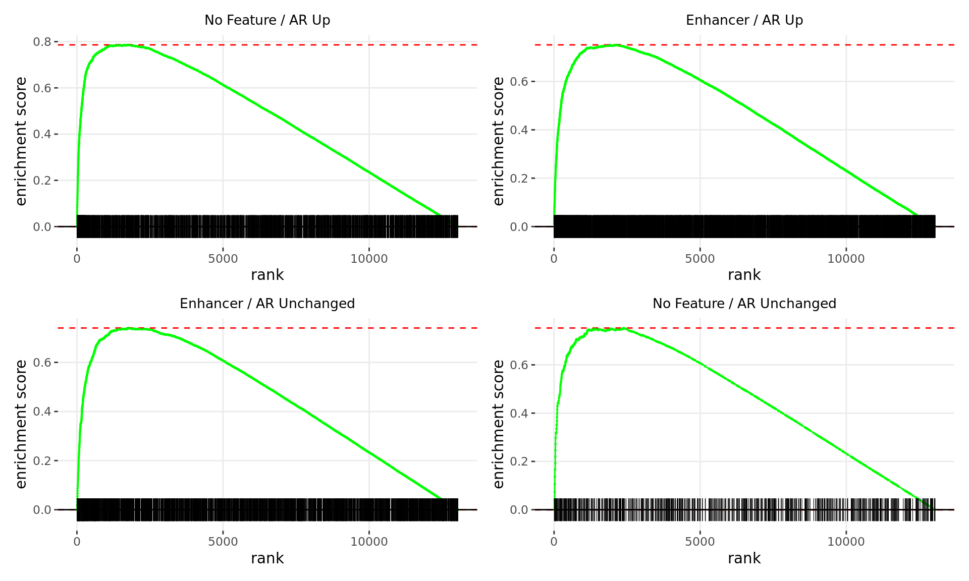
Merged windows were mapped to genes and their position amongst the RNA-Seq results was assessed. Windows were classified based on which feature was the best overlap, and the direction of AR binding with E2DHT treatment. 4 sets of windows were associated with overall changes in gene expression, using only the test statistic to rank the 13,043 genes considered as detected.
wrap_plots(p)
Barcode plots for the top 4 sets of windows associated with
nondirectional changes in gene expression.
The enrichment testing results from the AR differential binding
analysis were then compared to GSEA results obtained from the RNA-Seq
data set. Given the orthogonal nature of the two dataset, p-values from
each analysis were combined using Wilkinson’s maximum p-value method and
the resulting p-values adjusted as previously. Distances between nodes
(gene-sets) for all network plots were determined by using ChIP target
genes within the leading edge only.
Using the ranked list of genes from the RNA-Seq data, the 5 genes
most highly ranked for differential expression, with more than one
AR-bound window mapped to it were selected for visualisation.
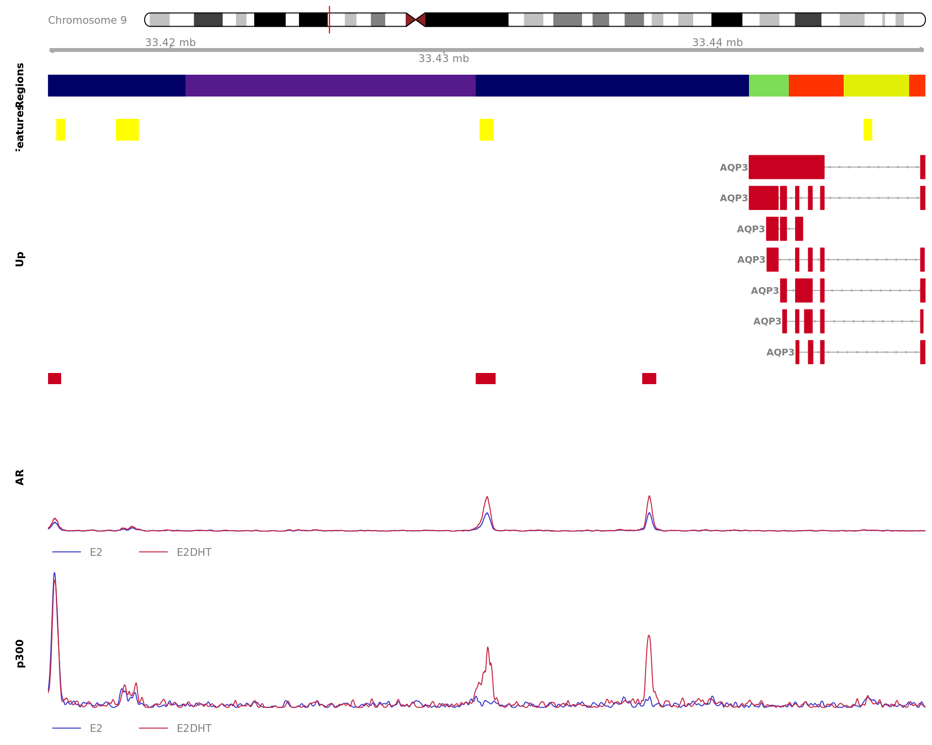
Region showing all merged AR-bound windows mapped to UGDH. Windows
considered to be unchanged for AR are annotated in grey, with other
colours indicating AR gain or loss. Mapped windows are only shown if
within 5Mb of UGDH. Gene-centric regions and external features are shown
in the top panel. The estimated logFC for UGDH is 1.52 with an FDR of
2.34e-10. Undetected and unchanged genes are shown on separate
tracks.
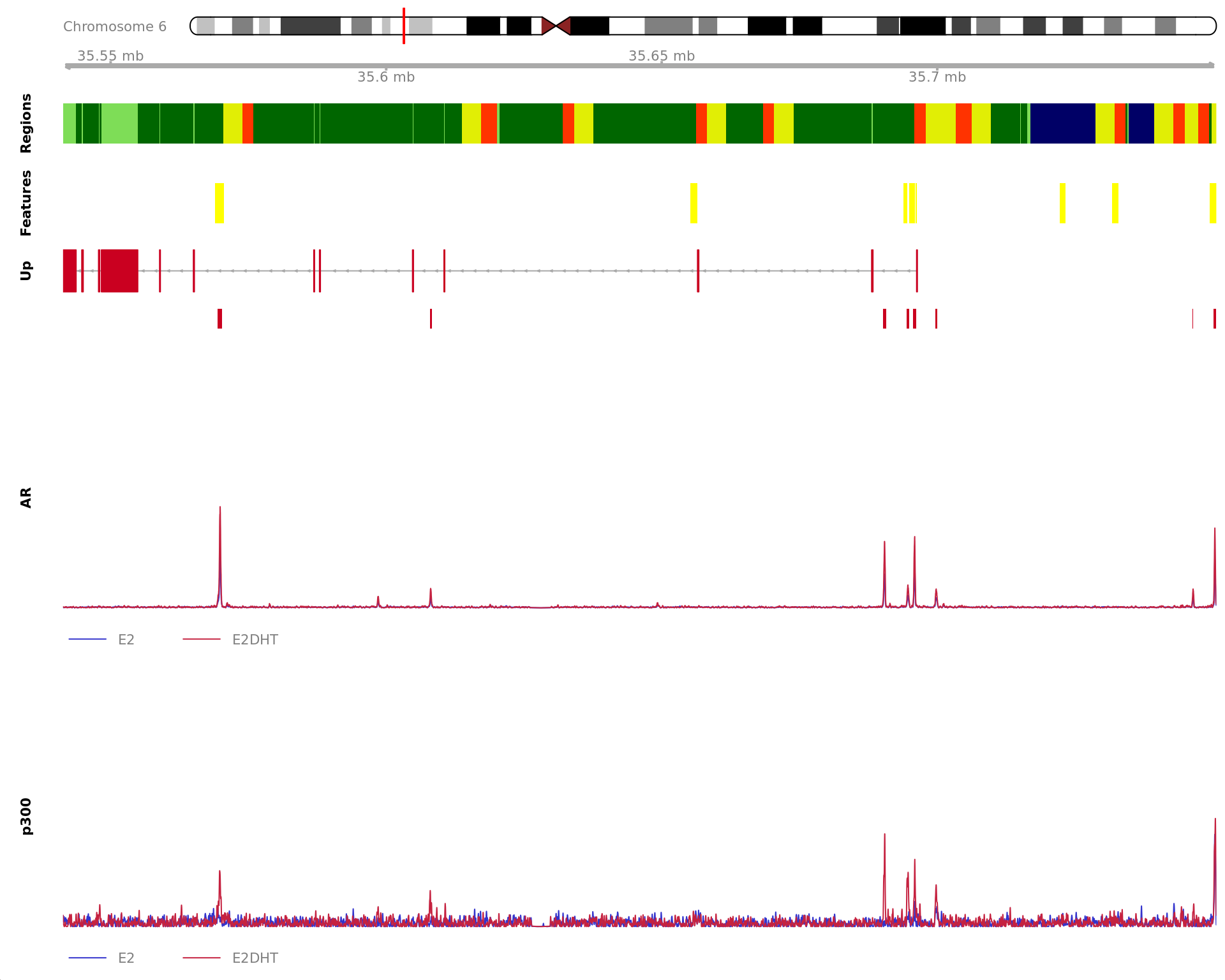
Region showing all merged AR-bound windows mapped to FKBP5. Windows
considered to be unchanged for AR are annotated in grey, with other
colours indicating AR gain or loss. Mapped windows are only shown if
within 5Mb of FKBP5. Gene-centric regions and external features are
shown in the top panel. The estimated logFC for FKBP5 is 2.00 with an
FDR of 6.51e-10. Undetected and unchanged genes are shown on separate
tracks.
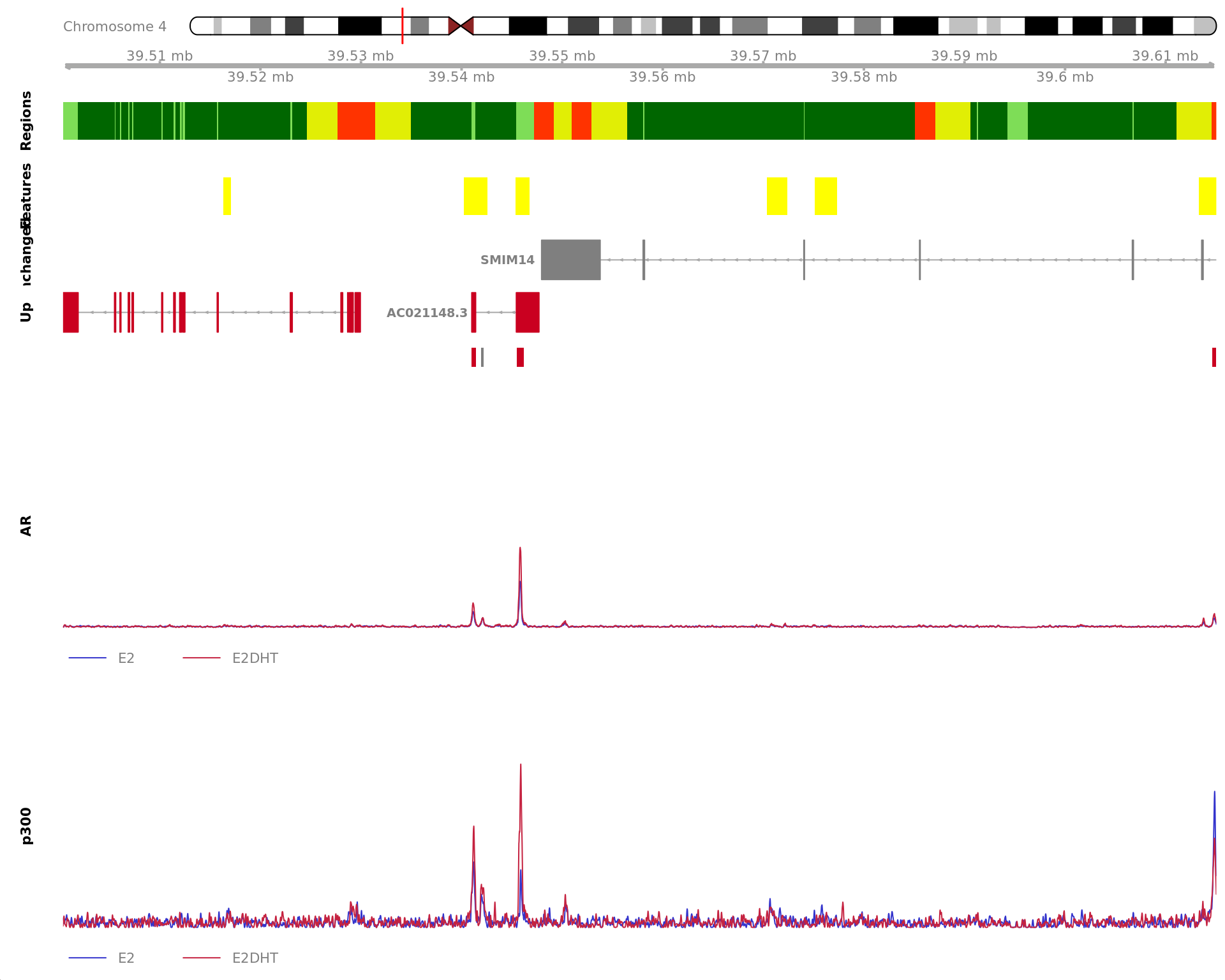
Region showing all merged AR-bound windows mapped to SEC14L2.
Windows considered to be unchanged for AR are annotated in grey, with
other colours indicating AR gain or loss. Mapped windows are only shown
if within 5Mb of SEC14L2. Gene-centric regions and external features are
shown in the top panel. The estimated logFC for SEC14L2 is 2.65 with an
FDR of 8.87e-10. Undetected and unchanged genes are shown on separate
tracks.
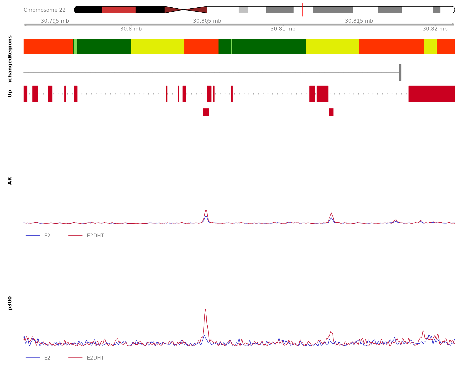
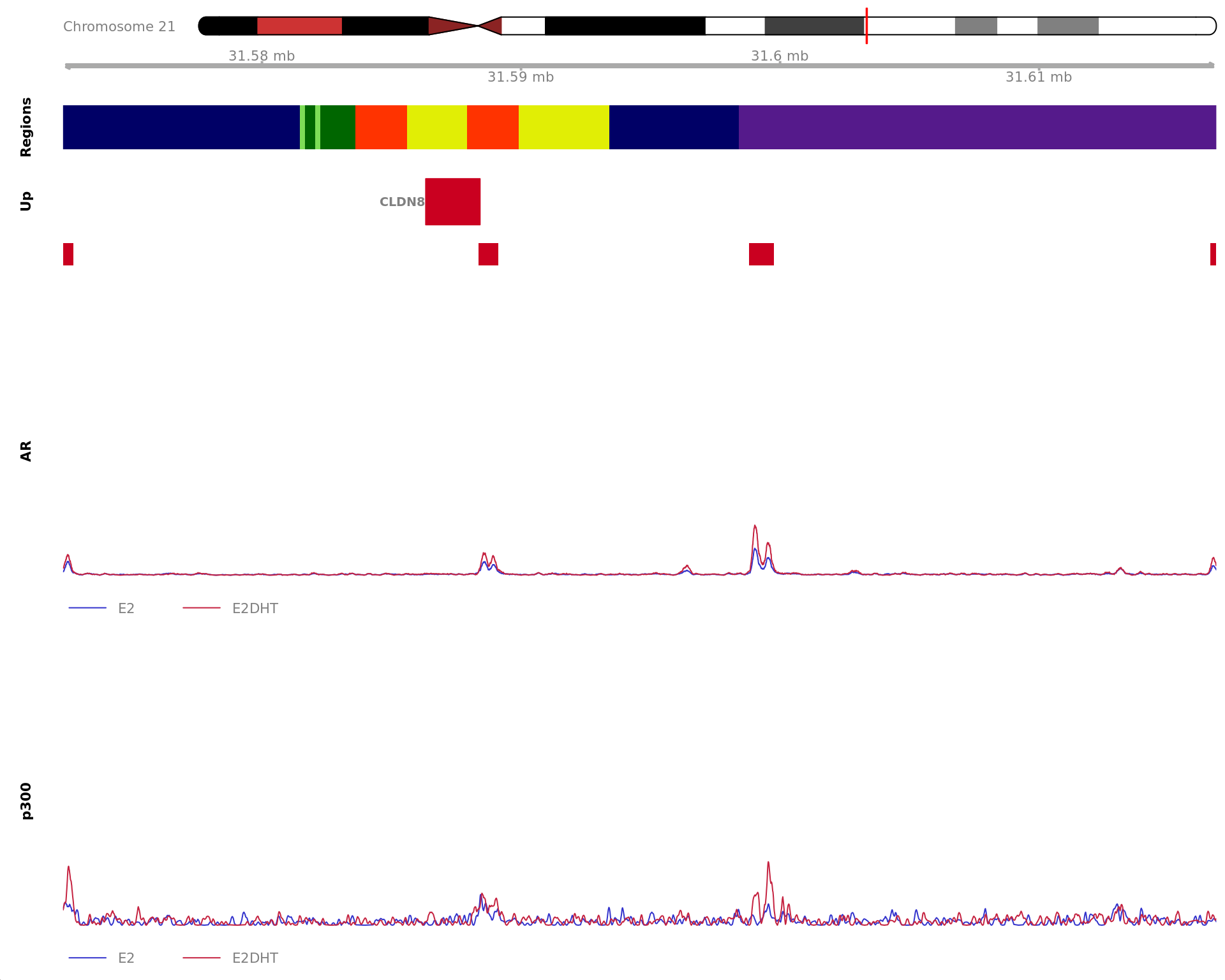
Region showing all merged AR-bound windows mapped to CLDN8. Windows
considered to be unchanged for AR are annotated in grey, with other
colours indicating AR gain or loss. Mapped windows are only shown if
within 5Mb of CLDN8. Gene-centric regions and external features are
shown in the top panel. The estimated logFC for CLDN8 is 2.31 with an
FDR of 1.01e-09. Undetected and unchanged genes are shown on separate
tracks.
Hicks, S. C., and R. A. Irizarry. 2015. “quantro: a data-driven approach to guide the choice of an
appropriate normalization method.”Genome Biol 16
(June): 117.
Hicks, Stephanie C, Kwame Okrah, Joseph N Paulson, John Quackenbush,
Rafael A Irizarry, and Héctor Corrada Bravo. 2017. “Smooth quantile normalization.”Biostatistics 19 (2): 185–98. https://doi.org/10.1093/biostatistics/kxx028.
Ignatiadis, N., B. Klaus, J. B. Zaugg, and W. Huber. 2016. “Data-driven hypothesis weighting increases
detection power in genome-scale multiple testing.”Nat
Methods 13 (7): 577–80.
Korotkevich, Gennady, Vladimir Sukhov, and Alexey Sergushichev. 2019.
“Fast Gene Set Enrichment Analysis.”bioRxiv. https://doi.org/10.1101/060012.
Law, C. W., Y. Chen, W. Shi, and G. K. Smyth. 2014. “voom: Precision weights unlock linear model
analysis tools for RNA-seq read
counts.”Genome Biol 15 (2): R29.
Lun, A. T., and G. K. Smyth. 2015. “From reads to regions: a
Bioconductor workflow to detect differential binding in
ChIP-seq data.”F1000Res 4: 1080.
Lun, Aaron T L, and Gordon K Smyth. 2014. “De Novo
Detection of Differentially Bound Regions for
ChIP-Seq Data Using Peaks and
Windows: Controlling Error Rates Correctly.”Nucleic Acids
Res. 42 (11): e95.
McCarthy, Davis J., and Gordon K. Smyth. 2009. “Testing significance relative to a fold-change threshold
is a TREAT.”Bioinformatics 25 (6): 765–71. https://doi.org/10.1093/bioinformatics/btp053.
Subramanian, Aravind, Pablo Tamayo, Vamsi K. Mootha, Sayan Mukherjee,
Benjamin L. Ebert, Michael A. Gillette, Amanda Paulovich, et al. 2005.
“Gene Set Enrichment Analysis: A Knowledge-Based Approach for
Interpreting Genome-Wide Expression Profiles.”Proceedings of
the National Academy of Sciences 102 (43): 15545–50. https://doi.org/10.1073/pnas.0506580102.
Young, M. D., M. J. Wakefield, G. K. Smyth, and A. Oshlack. 2010.
“Gene ontology analysis for
RNA-seq: accounting for selection
bias.”Genome Biol 11 (2): R14.
Zhang, Y., T. Liu, C. A. Meyer, J. Eeckhoute, D. S. Johnson, B. E.
Bernstein, C. Nusbaum, et al. 2008. “Model-based analysis of
ChIP-Seq
(MACS).”Genome Biol 9 (9): R137.