Motif Analysis Using motifTestR
Stevie Pederson
Black Ochre Data Labs, The Kids Research Institute Australiastephen.pederson.au@gmail.com Source:
vignettes/motifAnalysis.Rmd
motifAnalysis.RmdAbstract
Analysis of transcription factor binding motifs using Position Weight Matrices (PWMs) is a common task in analysis of genomic data. Two key tests for analysis of TFBMs using morifTestR are demonstrated below
Introduction
Bioinformatic analysis of data from ChIP-Seq or ATAC-Seq, along with multiple other approaches, can involve the analysis of sequences within the regions identified is being of interest. Whilst these analyses are not restricted to transcription factors, this can often form an important component of this type of analysis. Analysis of Transcription Factor Binding Motifs (TFBMs) is often performed using Position Weight Matrices (PWMs) to encode the flexibility in which exact sequence is bound by the particular transcription factor, and is a computationally demanding task with many popular tools enabling analysis outside of R.
The tools within motifTestR aim to build on and expand
the existing resources available to the Bioconductor community,
performing all analyses inside the R environment. The package offers two
complementary approaches to TFBM analysis within XStringSet
objects containing multiple sequences. The function
testMotifPos() identifies motifs showing positional
bias within a set of sequences, whilst overall enrichment
within a set of sequences is enabled by testMotifEnrich().
These are then extended to analyse motifs grouped into “clusters” using
testClusterPos() and testClusterEnrich().
Additional functions aid in the visualisation and preparation of these
two key approaches.
Setup
Installation
In order to perform the operations in this vignette, first install
motifTestR.
if (!"BiocManager" %in% rownames(installed.packages()))
  install.packages("BiocManager")
BiocManager::install("motifTestR")
Once installed, we can load all required packages, set a default plotting theme and setup how many threads to use during the analysis.
library(motifTestR)
library(rtracklayer)
library(BSgenome.Hsapiens.UCSC.hg19)
library(parallel)
library(ggplot2)
library(patchwork)
library(universalmotif)
library(extraChIPs)
theme_set(theme_bw())
cores <- 1
Defining a Set of Peaks
The peaks used in this workflow were obtained from the bed files
denoting binding sites of the Androgen Receptor and Estrogen Receptor
along with H3K27ac marks, in ZR-75-1 cells under DHT treatment (Hickey et al. 2021). The object
ar_er_peaks contains a subset of 849 peaks found within
chromosome 1, with all peaks resized to 400bp
data("ar_er_peaks")
ar_er_peaks
## GRanges object with 849 ranges and 0 metadata columns:
## seqnames ranges strand
## <Rle> <IRanges> <Rle>
## [1] chr1 1008982-1009381 *
## [2] chr1 1014775-1015174 *
## [3] chr1 1051296-1051695 *
## [4] chr1 1299561-1299960 *
## [5] chr1 2179886-2180285 *
## ... ... ... ...
## [845] chr1 246771887-246772286 *
## [846] chr1 246868678-246869077 *
## [847] chr1 246873126-246873525 *
## [848] chr1 247095351-247095750 *
## [849] chr1 247267507-247267906 *
## -------
## seqinfo: 24 sequences from hg19 genome
sq <- seqinfo(ar_er_peaks)Whilst the example dataset is small for the convenience of an R package, those wishing to work on the complete set of peaks (i.e. not just chromosome 1) may run the code provided in the final section to obtain all peaks. This will produce a greater number of significant results in subsequent analyses but will also increase running times for all functions.
Obtaining a Set of Sequences for Testing
Now that we have genomic co-ordinates as a set of peaks, we can obtain the sequences that are associated with each peak. The source ranges can optionally be added to the sequences as names by coercing the ranges to a character vector.
test_seq <- getSeq(BSgenome.Hsapiens.UCSC.hg19, ar_er_peaks)
names(test_seq) <- as.character(ar_er_peaks)
Obtaining a List of PWMs for Testing
A small list of Position Frequency Matrices (PFMs), obtained from MotifDb are provided with the package and these will be suitable for all downstream analysis. All functions will convert PFMs to PWMs internally.
## [1] "ESR1" "ANDR" "FOXA1" "ZN143" "ZN281"
ex_pfm$ESR1## 1 2 3 4 5 6 7 8 9 10 11 12 13
## A 0.638 0.074 0.046 0.094 0.002 0.856 0.108 0.396 0.182 0.104 0.054 0.618 0.040
## C 0.048 0.006 0.018 0.072 0.888 0.006 0.442 0.604 0.376 0.078 0.034 0.198 0.884
## G 0.260 0.808 0.908 0.178 0.048 0.112 0.312 0.000 0.286 0.044 0.908 0.070 0.014
## T 0.054 0.112 0.028 0.656 0.062 0.026 0.138 0.000 0.156 0.774 0.004 0.114 0.062
## 14 15
## A 0.090 0.058
## C 0.822 0.330
## G 0.008 0.066
## T 0.080 0.546Again, a larger set of motifs may be obtained using or modifying the example code at the end of the vignette
Searching Sequences
Finding PWM Matches
All PWM matches within the test sequences can be returned for any of
the PWMs, with getPwmMatches() searching using the PWM and
it’s reverse complement by default. Matches are returned showing their
position within the sequence, as well as the distance from the centre of
the sequence and the matching section within the larger sequence. Whilst
there is no strict requirement for sequences of the same width,
generally this is good practice for this type of analysis and is
commonly a requirement for downstream statistical analysis.
score_thresh <- "70%"
getPwmMatches(ex_pfm$ESR1, test_seq, min_score = score_thresh)
## DataFrame with 51 rows and 8 columns
## seq score direction start end from_centre
## <character> <numeric> <factor> <integer> <integer> <numeric>
## 1 chr1:1008982-1009381 17.3522 R 216 230 23
## 2 chr1:6543164-6543563 15.7958 R 176 190 -17
## 3 chr1:10010470-10010869 18.0880 F 193 207 0
## 4 chr1:11434290-11434689 20.8412 R 321 335 128
## 5 chr1:17855904-17856303 15.7429 F 195 209 2
## ... ... ... ... ... ... ...
## 47 chr1:212731397-21273.. 16.1154 R 88 102 -105
## 48 chr1:214500812-21450.. 17.1325 R 186 200 -7
## 49 chr1:217979498-21797.. 16.6438 F 186 200 -7
## 50 chr1:233243433-23324.. 15.7178 F 201 215 8
## 51 chr1:247267507-24726.. 16.8796 F 313 327 120
## seq_width match
## <integer> <DNAStringSet>
## 1 400 TGGTCACAGTGACCT
## 2 400 GGGTCATCCTGTCCC
## 3 400 AGGTCACCCTGGCCC
## 4 400 AGGTCACCGTGACCC
## 5 400 AGGGCAAAATGACCC
## ... ... ...
## 47 400 GTGTCACAGTGACCC
## 48 400 AGGTCACAATGACAT
## 49 400 GGGTCATCCTGCCCC
## 50 400 AGGTCATAAAGACCT
## 51 400 AGGTCAGAATGACCGMany sequences will contain multiple matches, and we can subset our
results to only the ‘best match’ by setting
best_only = TRUE. The best match is chosen by the highest
score returned for each match. If multiple matches return identical
scores, all tied matches are returned by default and will be equally
down-weighted during positional analysis. This can be further controlled
by setting break_ties to any of c(“random”, “first”,
“last”, “central”), which will choose randomly, by sequence order or
proximity to centre.
getPwmMatches(ex_pfm$ESR1, test_seq, min_score = score_thresh, best_only = TRUE)## DataFrame with 50 rows and 8 columns
## seq score direction start end from_centre
## <character> <numeric> <factor> <integer> <integer> <numeric>
## 1 chr1:1008982-1009381 17.3522 R 216 230 23
## 2 chr1:6543164-6543563 15.7958 R 176 190 -17
## 3 chr1:10010470-10010869 18.0880 F 193 207 0
## 4 chr1:11434290-11434689 20.8412 R 321 335 128
## 5 chr1:17855904-17856303 15.7429 F 195 209 2
## ... ... ... ... ... ... ...
## 46 chr1:212731397-21273.. 16.1154 R 88 102 -105
## 47 chr1:214500812-21450.. 17.1325 R 186 200 -7
## 48 chr1:217979498-21797.. 16.6438 F 186 200 -7
## 49 chr1:233243433-23324.. 15.7178 F 201 215 8
## 50 chr1:247267507-24726.. 16.8796 F 313 327 120
## seq_width match
## <integer> <DNAStringSet>
## 1 400 TGGTCACAGTGACCT
## 2 400 GGGTCATCCTGTCCC
## 3 400 AGGTCACCCTGGCCC
## 4 400 AGGTCACCGTGACCC
## 5 400 AGGGCAAAATGACCC
## ... ... ...
## 46 400 GTGTCACAGTGACCC
## 47 400 AGGTCACAATGACAT
## 48 400 GGGTCATCCTGCCCC
## 49 400 AGGTCATAAAGACCT
## 50 400 AGGTCAGAATGACCGWe can return all matches for a complete list of PWMs, as a list of DataFrame objects. This strategy allows for visualisation of results as well as testing for positional bias.
bm_all <- getPwmMatches(
  ex_pfm, test_seq, min_score = score_thresh, best_only = TRUE, break_ties = "all",
  mc.cores = cores
)
This same strategy of passing a single, or multiple PWMs can be applied even when simply wishing to count the total matches for each PWM. Counting may be useful for restricting downstream analysis to the set of motifs with more than a given number of matches.
countPwmMatches(ex_pfm, test_seq, min_score = score_thresh, mc.cores = cores)## ESR1 ANDR FOXA1 ZN143 ZN281
## 51 36 292 43 46Analysis of Positional Bias
Testing for Positional Bias
A commonly used tool within the MEME-Suite is centrimo
(Bailey and Machanick 2012) and
motifTestR provides a simple, easily interpretable
alternative approach using testMotifPos(). This function
bins the distances from the centre of each sequence with the central bin
being symmetrical around zero, and if no positional bias is expected
(i.e. H0), matches should be equally distributed between
bins. Unlike centrimo, no assumption of centrality
is made and any notable deviations from a discrete uniform distribution
may be considered as significant.
A test within each bin is performed using binom.test()
and a single, summarised p-value across all bins is returned using the
asymptotically exact harmonic mean p-value (HMP) (Wilson 2019). By default, the binomial test is
applied for the null hypothesis to detect matches in each bin which are
greater than expected, however, this can also be set by the
user. When using the harmonic-mean p-value however, choosing the
alternate hypothesis as “greater” tends return a more conservative
p-value across the entire set of bins.
res_pos <- testMotifPos(bm_all, mc.cores = cores)
head(res_pos)
## start end centre width total_matches matches_in_region expected
## ESR1 5 15 10 10 50 8 1.291990
## ANDR -25 -5 -15 20 34 12 1.770833
## FOXA1 -5 25 10 30 238 32 12.205128
## ZN143 -55 55 0 110 26 20 5.473684
## ZN281 -195 195 0 390 40 38 25.529716
## enrichment prop_total p fdr consensus_motif
## ESR1 6.192000 0.1600000 0.001643146 0.008215728 35, 0, 1....
## ANDR 6.776471 0.3529412 0.004700634 0.011751585 0, 0, 0,....
## FOXA1 2.621849 0.1344538 0.010576124 0.017626873 0, 0, 0,....
## ZN143 3.653846 0.7692308 0.243171867 0.303964834 6, 1, 13....
## ZN281 1.488462 0.9500000 0.977504172 0.977504172 8, 6, 22....The bins returned by the function represent the widest range of bins
where the raw p-values were below the HMP. Wide ranges tend to be
associated with lower significance for a specific PWM. This is a further
point of divergence from centrimo in that results are
dependent on the pre-determined bin-size and the region of enrichment is
formed using p-values, instead of the adaptive methods of
centrimo (Bailey and Machanick
2012).
Due to the two-stranded nature of DNA, the distance from zero can
also be assessed by setting abs = TRUE and in this case the
first bin begins at zero.
res_abs <- testMotifPos(bm_all, abs = TRUE, mc.cores = cores)
head(res_abs)
## start end centre width total_matches matches_in_region expected
## ESR1 10 20 15 10 50 11 2.590674
## ANDR 10 20 15 10 34 8 1.770833
## FOXA1 0 30 15 30 238 69 36.615385
## ZN143 0 50 25 50 26 20 6.842105
## ZN281 0 190 95 190 40 38 33.160622
## enrichment prop_total p fdr consensus_motif
## ESR1 4.246000 0.2200000 0.0007907262 0.003953631 35, 0, 1....
## ANDR 4.517647 0.2352941 0.0057468643 0.014367161 0, 0, 0,....
## FOXA1 1.884454 0.2899160 0.0106210602 0.017701767 0, 0, 0,....
## ZN143 2.923077 0.7692308 0.1963203926 0.245400491 6, 1, 13....
## ZN281 1.145938 0.9500000 0.9173293626 0.917329363 8, 6, 22....This approach is particularly helpful for detecting co-located transcription factors which can be any distance from the TF which was used to obtain and centre the test set of sequences.
Viewing Matches
The complete set of matches returned as a list above can be simply
passed to ggplot2 (Wickham
2016) for visualisation, in order to asses whether any PWM
appears to have a positional bias. By default, smoothed values across
all motifs will be overlaid (Figure 1A), however, tailoring using ggplot
is simple to produce a wide variety of outputs (Figure 1B)
topMotifs <- res_pos |>
    subset(fdr < 0.05) |>
    rownames()
A <- plotMatchPos(bm_all[topMotifs], binwidth = 10, se = FALSE)
B <- plotMatchPos(
    bm_all[topMotifs], binwidth = 10, geom = "col", use_totals = TRUE
) +
  geom_smooth(se = FALSE, show.legend = FALSE) +
  facet_wrap(~name)
A + B + plot_annotation(tag_levels = "A") & theme(legend.position = "bottom")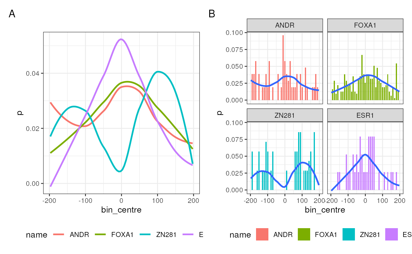
Distribution of motif matches around the centres of the set of peaks
Whilst the above will produce figures showing the symmetrical distribution around the peak centres, the distance from the peak centre can also be shown as an absolute distance. In Figure 2 distances shown as a heatmap (A) or as a CDF (B). The latter makes it easy to see that 50% of ESR1 matches occur within a short distance of the centre (~25bp), whilst for ANDR and FOXA1, this distance is roughly doubled. Changing the binwidth argument can either smooth data or increase the fine resolution.
topMotifs <- res_abs |>
    subset(fdr < 0.05) |>
    rownames()
A <- plotMatchPos(bm_all[topMotifs], abs = TRUE, type = "heatmap") +
  scale_fill_viridis_c()
B <- plotMatchPos(
  bm_all[topMotifs], abs = TRUE, type = "cdf", geom = "line", binwidth = 5
)
A + B + plot_annotation(tag_levels = "A") & theme(legend.position = "bottom")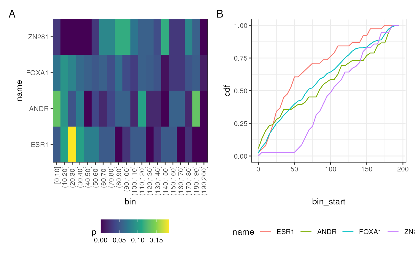
Distribution of motif matches shown as a distance from the centre of each sequence
Testing For Motif Enrichment
As well as providing methods for analysing positional bias within a
set of PWM matches, methods to test for enrichment are also implemented
in motifTestR. A common approach when testing for motif
enrichment is to obtain a set of random or background sequences which
represent a suitable control set to define the null hypothesis
(H0). In motifTestR, two alternatives are
offered utilising this approach, which both return similar results but
involve different levels of computational effort.
The first approach is to sample multiple sets of background sequences
and by ‘iterating’ through to obtain a null distribution for PWM matches
and comparing our observed counts against this distribution. It has been
noticed that this approach commonly produces a set of counts for
H0 which closely resemble a Poisson distribution, and a
second approach offered in motifTestR is to sample a
suitable large set of background sequences and estimate the parameters
for the Poisson distribution for each PWM, and testing against
these.
Defining a Set of Control Sequences
Choosing a suitable set of control sequences can be undertaken by any
number of methods. motifTestR enables a strategy of
matching sequences by any number of given features. The data object
zr75_enh contains the candidate enhancers for ZR-75-1 cells
defined by v2.0 of the Enhancer Atlas (Gao and
Qian 2019), for chromosome 1 only. A high proportion of our peaks
are associated with these regions and choosing control sequences drawn
from the same proportion of these regions may be a viable strategy.
data("zr75_enh")
mean(overlapsAny(ar_er_peaks, zr75_enh))
## [1] 0.6914016First we can annotate each peak by whether there is any overlap with an enhancer, or whether the peak belongs to any other region. Next we can define two sets of GenomicRanges, one representing the enhancers and the other being the remainder of the genome, here restricted to chromosome 1 for consistency. Control regions can be drawn from each with proportions that match the test set of sequences.
ar_er_peaks$feature <- ifelse(
  overlapsAny(ar_er_peaks, zr75_enh), "enhancer", "other"
)
chr1 <- GRanges(sq)[1]
bg_ranges <- GRangesList(
  enhancer = zr75_enh,
  other = GenomicRanges::setdiff(chr1, zr75_enh)
)
The provided object hg19_mask contains regions of the
genome which are rich in Ns, such as centromeres and telomeres.
Sequences containing Ns produce warning messages when matching PWMs and
avoiding these regions may be wise, without introducing any sequence
bias. These are then passed to makeRMRanges() as ranges to
be excluded, whilst sampling multiple random, size-matched ranges
corresponding to our test set of ranges with sequences being analysed,
and drawn proportionally from matching genomic regions. Whilst our
example only used candidate enhancers, any type and number of genomic
regions can be used, with a limitless number of classification
strategies being possible.
data("hg19_mask")
set.seed(305)
rm_ranges <- makeRMRanges(
  splitAsList(ar_er_peaks, ar_er_peaks$feature),
  bg_ranges, exclude = hg19_mask,
  n_iter = 100
)
This has now returned a set of control ranges which are
randomly-selected (R) size-matched (M) to our peaks and are drawn from a
similar distribution of genomic features. By setting
n_iter = 100, this set will be 100 times larger than our
test set and typically this value can be set to 1000 or even 5000 for
better estimates of parameters under the null distribution. However,
this will increase the computational burden for analysis.
If not choosing an iterative strategy, a total number of sampled
ranges can also be specified. In this case the column
iteration will not be added to the returned ranges.
In order to perform the analysis, we can now extract the genomic
sequences corresponding to our randomly selected control ranges. Passing
the mcols element ensure the iteration numbers are passed
to the sequences, as these are required for this approach.
If choosing strategies for enrichment testing outside of
motifTestR, these sequences can be exported as a fasta file
using writeXStringSet from the Biostrings
package.
Testing For Enrichment
Testing for overall motif enrichment is implemented using multiple strategies, using Poisson, QuasiPoisson or pure Iterative approaches. Whilst some PWMs may closely follow a Poisson distribution under H0, others may be over-dispersed and more suited to a Quasi-Poisson approach. Each approach has unique advantages and weaknesses as summarised below:
-
Poisson
- Can use any number of BG Sequences, unrelated to the test set
- Modelling is performed based on the expected number of matches per sequence
- The fastest approach
- Anti-conservative p-values where counts are over-dispersed
- Appropriate for “quick & dirty” checks for expected discoveries
-
QuasiPoisson
- Modelling is performed per set of sequences (of identical size to the test set)
- Requires BG Sequences to be in ‘iterative’ blocks
- Fewer ‘iterative blocks’ can still model over-dispersion reasonably well
-
Iterative
- No model assumptions
- Requires BG Sequences to be in ‘iterative’ blocks
- P-Values derived from Z-scores (using the Central Limit Theorem)
- Sampled p-values from iterations can be used if preferred
- Requires the largest number of iterative blocks (>1000)
- Slowest, but most reliable approach
From a per iteration perspective there is little difference between the Iterative and the modelled QuasiPoisson approaches, however the modelled approaches can still return reliable results from a lower number of iterative blocks, lending a clear speed advantage. Z-scores returned are only used for statistical testing under the iterative approach and are for indicative purposes only under all other models model.
Whilst no guidelines have been developed for an optimal number of sequences, a control set which is orders of magnitude larger than the test set may be prudent. A larger set of control sequences clearly leads to longer analytic time-frames and larger computational resources, so this is left to what is considered appropriate by the researcher, nothing that here, we chose a control set which is 100x larger than our test sequences. If choosing an iterative approach and using the iteration-derived p-values, setting a number of iterations based on the resolution required for these values may be important, noting that the lowest possible p-value is 1/n_iterations.
enrich_res <- testMotifEnrich(
  ex_pfm, test_seq, rm_seq, min_score = score_thresh, model = "quasi", mc.cores = cores
)
head(enrich_res)
## sequences matches expected enrichment Z p fdr
## ZN143 849 43 1.22 35.245902 38.737822 1.585282e-37 7.926411e-37
## ESR1 849 51 5.40 9.444444 20.012479 1.734768e-28 4.336921e-28
## FOXA1 849 293 126.60 2.314376 13.299432 1.188963e-22 1.981605e-22
## ANDR 849 36 12.60 2.857143 6.290326 4.520855e-08 5.651069e-08
## ZN281 849 47 20.62 2.279340 4.852750 9.665125e-06 9.665125e-06
## n_iter sd_bg
## ZN143 100 1.078532
## ESR1 100 2.278578
## FOXA1 100 12.511813
## ANDR 100 3.719998
## ZN281 100 5.436093Setting the model to “iteration” instead uses a classical iterative approach to define the null distributions of counts and Z-scores are calculated from these values. The returned p-values from this test are taken from the Z-scores directly, with p-values derived from the sampled iterations also returned if preferred for use in results by the researcher. Whilst requiring greater computational effort, fewer statistical assumptions are made and results may be more conservative than under modelling approaches.
iter_res <- testMotifEnrich(
  ex_pfm, test_seq, rm_seq, min_score = score_thresh, mc.cores = cores, model = "iteration"
)
head(iter_res)
## sequences matches expected enrichment Z p
## ESR1 849 52 5.41 9.611830 21.469841 0.000000e+00
## FOXA1 849 293 126.64 2.313645 13.345825 0.000000e+00
## ZN143 849 44 1.19 36.974790 102.144041 0.000000e+00
## ANDR 849 37 12.53 2.952913 7.014137 2.313705e-12
## ZN281 849 47 20.53 2.289333 5.186250 2.145708e-07
## fdr iter_p n_iter sd_bg
## ESR1 0.000000e+00 0.01 100 2.170021
## FOXA1 0.000000e+00 0.01 100 12.465322
## ZN143 0.000000e+00 0.01 100 0.419114
## ANDR 2.892131e-12 0.01 100 3.488669
## ZN281 2.145708e-07 0.01 100 5.103880Once we have selected our motifs of interest, sequences with matches
can be compared to easily assess co-occurrence, using
plotOverlaps() from extraChIPs.
In our test set, peaks were selected based on co-detection of ESR1 and
ANDR, however the rate of co-occurrence is low, revealing key insights
into the binding dynamics of these two TFs.
ex_pfm |>
  getPwmMatches(test_seq, min_score = score_thresh, mc.cores = cores) |>
  lapply(\(x) x$seq) |>
  plotOverlaps(type = "upset")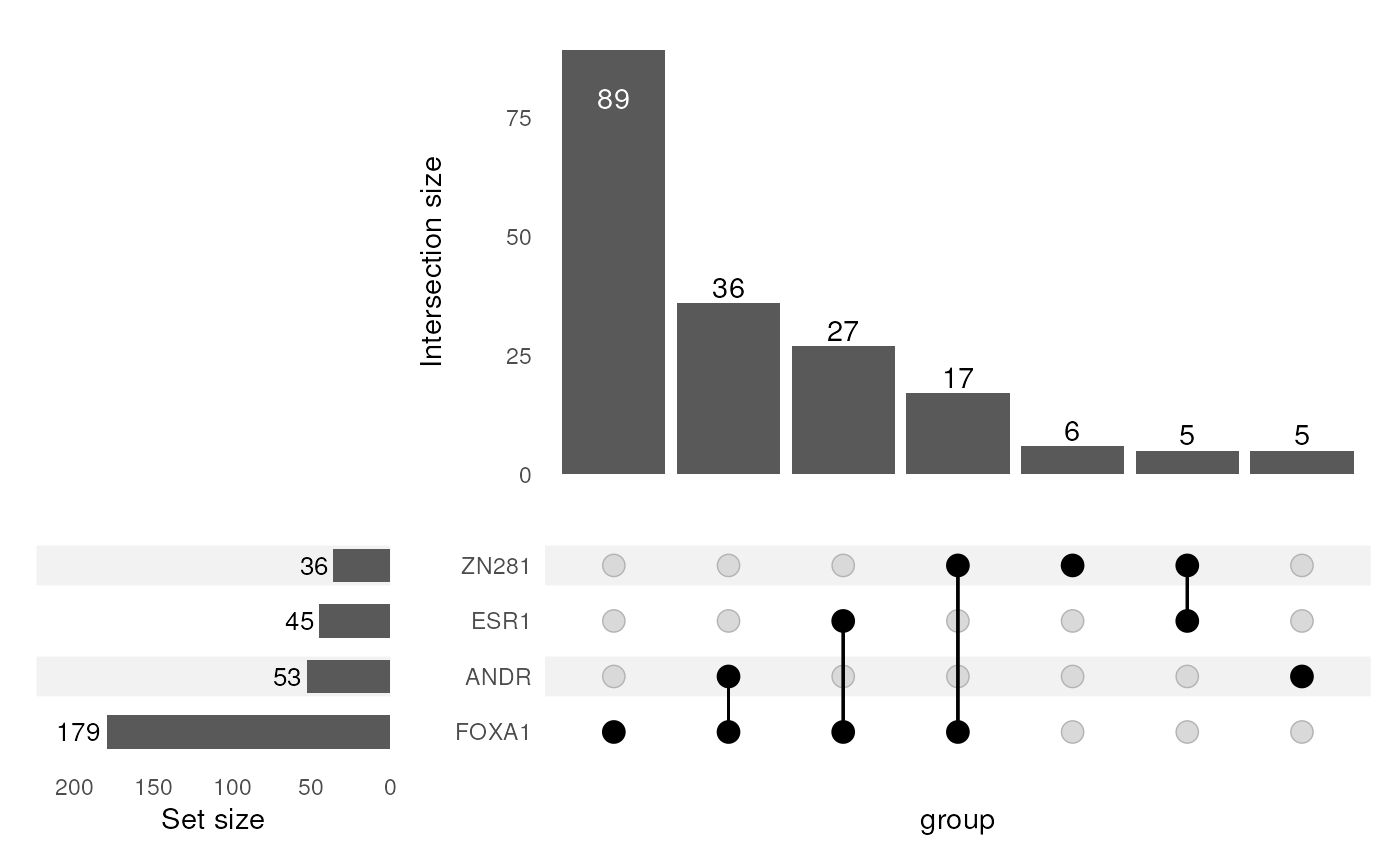
Distribution of select PWM matches within sequences. Each sequence is only considered once and as such, match numbers may be below those returned during testing, which includes multiple matches within a sequence.
Working with Clustered Motifs
TFBMs often contain a high level of similarity to other TFBMs, especially those within large but closely related families, such as the GATA or STAT families. It can be difficult to ascertain which member of a family is truly bound to a site from inspecting the sequence data alone.
As a relevant example, when looking at the above UpSet plot, about half of the sequences where a match to the ANDR motif was found also contain a FOXA1 motif. Does this mean that both are bound to the sequence, or have the same sequences simply been matched to both PWMs? As we can see there is quite some similarity in the core regions of the two binding motifs
c("ANDR", "FOXA1") |>
    lapply(
        \(x) create_motif(ex_pfm[[x]], name = x, type = "PPM")
    ) |>
    view_motifs()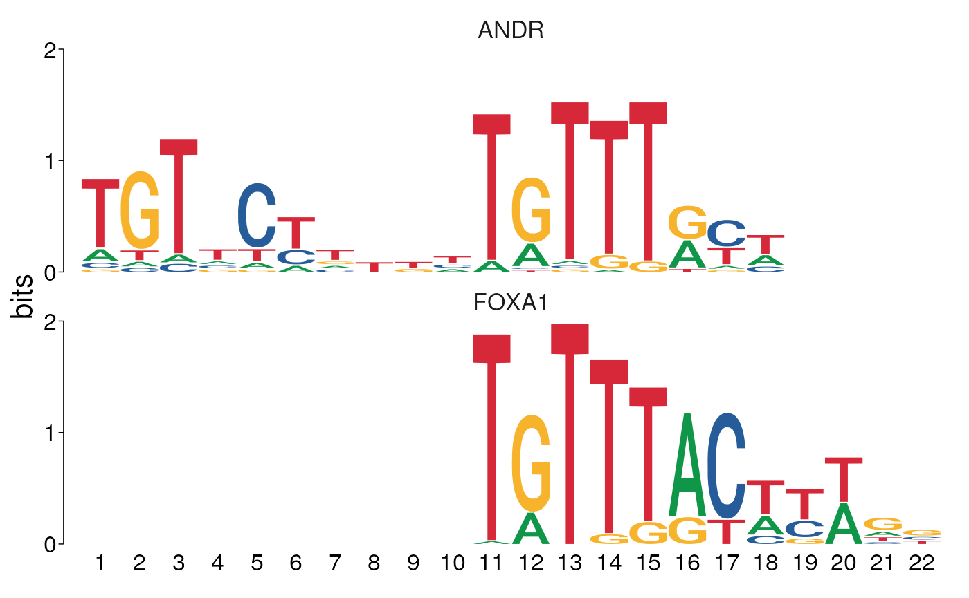
Binding Motifs for ANDR and FOXA1 overlaid for the best alignment, showing the similarity in the core regions.
motifTestR offers a simple but helpful strategy for
reducing the level of redundancy within a set of results, by grouping
highly similar motifs into a cluster and testing for
enrichment, or positional bias for any TFBM within that cluster. The
clustering methodology enabled within motifTestR allows for
the use of any of the comparison methods provided in
compare_motifs() (Tremblay
2024).
Whilst the example set of TFBMs is slightly artificial motifs can still be grouped into clusters. If using a larger database of TFBMs a carefully selected threshold may be more appropriate, however for this dataset, four clusters are able to be formed using the default settings. There is no ideal method to group PWMs into clusters and manual inspection of any clusters produced is the best strategy for this process. Names are not strictly required for downstream analysis, but can help with interpretability
cl <- clusterMotifs(ex_pfm, plot = TRUE, labels = NULL)
Plot produced when requested by clusterMotifs showing the relationship
between motifs. The red horizontal line indicates the threshold below
which motifs are grouped together into a cluster. Clustering is
performed using hclust on the distance matrices produced by
universalmotif::compare_motifs()
ex_cl <- split(ex_pfm, cl)
names(ex_cl) <- vapply(split(names(cl), cl), paste, character(1), collapse = "/")
These clusters can now be tested for positional bias using
testClusterPos(). Matches are the unique sites with a match
to any PWM within the cluster, and any overlapping sites from
matches to multiple PWMs are counted as a single match. When overlapping
matches are found, the one with the highest relative score (score /
maxScore) is chosen given that raw scores for each PWM will be on
different scales. A list of best matches can be produced in an
analogous way to for individual PWMs, using
getClusterMatches() instead of
getPwmMatches(), and the motif assigned to each match is
also provided.
cl_matches <- getClusterMatches(
    ex_cl, test_seq, min_score = score_thresh, best_only = TRUE
)
cl_matches
## $ESR1
## DataFrame with 50 rows and 9 columns
## seq score direction start end from_centre
## <character> <numeric> <factor> <integer> <integer> <numeric>
## 1 chr1:1008982-1009381 17.3522 R 216 230 23
## 2 chr1:6543164-6543563 15.7958 R 176 190 -17
## 3 chr1:10010470-10010869 18.0880 F 193 207 0
## 4 chr1:11434290-11434689 20.8412 R 321 335 128
## 5 chr1:17855904-17856303 15.7429 F 195 209 2
## ... ... ... ... ... ... ...
## 46 chr1:212731397-21273.. 16.1154 R 88 102 -105
## 47 chr1:214500812-21450.. 17.1325 R 186 200 -7
## 48 chr1:217979498-21797.. 16.6438 F 186 200 -7
## 49 chr1:233243433-23324.. 15.7178 F 201 215 8
## 50 chr1:247267507-24726.. 16.8796 F 313 327 120
## seq_width motif match
## <integer> <character> <DNAStringSet>
## 1 400 ESR1 TGGTCACAGTGACCT
## 2 400 ESR1 GGGTCATCCTGTCCC
## 3 400 ESR1 AGGTCACCCTGGCCC
## 4 400 ESR1 AGGTCACCGTGACCC
## 5 400 ESR1 AGGGCAAAATGACCC
## ... ... ... ...
## 46 400 ESR1 GTGTCACAGTGACCC
## 47 400 ESR1 AGGTCACAATGACAT
## 48 400 ESR1 GGGTCATCCTGCCCC
## 49 400 ESR1 AGGTCATAAAGACCT
## 50 400 ESR1 AGGTCAGAATGACCG
##
## $`ANDR/FOXA1`
## DataFrame with 255 rows and 9 columns
## seq score direction start end from_centre
## <character> <numeric> <factor> <integer> <integer> <numeric>
## 1 chr1:5658040-5658439 13.7470 R 203 214 8.5
## 2 chr1:6969924-6970323 14.0694 F 199 210 4.5
## 3 chr1:8077594-8077993 12.6907 F 28 39 -166.5
## 4 chr1:8121343-8121742 14.4605 F 177 188 -17.5
## 5 chr1:8130962-8131361 15.1441 F 341 352 146.5
## ... ... ... ... ... ... ...
## 251 chr1:241913254-24191.. 12.3147 F 196 207 1.5
## 252 chr1:244065451-24406.. 13.4339 R 288 299 93.5
## 253 chr1:244417385-24441.. 23.0102 R 167 184 -24.5
## 254 chr1:244490601-24449.. 16.6073 F 189 206 -2.5
## 255 chr1:246746473-24674.. 14.3461 F 40 51 -154.5
## seq_width motif match
## <integer> <character> <DNAStringSet>
## 1 400 FOXA1 TGTTTATTCTGT
## 2 400 FOXA1 TGTTTGCTTTTG
## 3 400 FOXA1 TGTGTACTTAGC
## 4 400 FOXA1 TGTTTACTTTCC
## 5 400 FOXA1 TGTTTATTTAGG
## ... ... ... ...
## 251 400 FOXA1 TGTTTATTTTAA
## 252 400 FOXA1 TATTTACTGTGG
## 253 400 ANDR TGTTCTTTTTTGTTTGTT
## 254 400 ANDR TGTTCTTTCGTGTTTGAC
## 255 400 FOXA1 TGTTTACTTTCT
##
## $ZN143
## DataFrame with 26 rows and 9 columns
## seq score direction start end from_centre
## <character> <numeric> <factor> <integer> <integer> <numeric>
## 1 chr1:1051296-1051695 24.3993 F 360 381 170.5
## 2 chr1:6673482-6673881 24.5459 R 199 220 9.5
## 3 chr1:10532432-10532831 26.8427 F 166 187 -23.5
## 4 chr1:22109982-22110381 29.0591 F 210 231 20.5
## 5 chr1:36614982-36615381 23.8117 R 243 264 53.5
## ... ... ... ... ... ... ...
## 22 chr1:224544286-22454.. 28.4852 R 151 172 -38.5
## 23 chr1:243418636-24341.. 22.4081 F 206 227 16.5
## 24 chr1:243419063-24341.. 24.5149 F 143 164 -46.5
## 25 chr1:244615397-24461.. 28.9222 R 166 187 -23.5
## 26 chr1:244815816-24481.. 30.0534 F 216 237 26.5
## seq_width motif match
## <integer> <character> <DNAStringSet>
## 1 400 ZN143 AGCGCCCTGGGAAATGTAGTCC
## 2 400 ZN143 TGCCTTGTGGGAGTGGTAGTCC
## 3 400 ZN143 AGCCTGCCGGGAGATGTAGTTC
## 4 400 ZN143 GGCATGCTGGGATTTGTAGTCT
## 5 400 ZN143 AGCACTCCGGGAGTTGTAGTTG
## ... ... ... ...
## 22 400 ZN143 CGCATGCTGGGAATTGTAGTTC
## 23 400 ZN143 GGCATGCTAGGAGTTGTAGTGT
## 24 400 ZN143 TGGTTTCTGGGAATTGTAGTGT
## 25 400 ZN143 TGCATGCTGGGATTTGTAGTCC
## 26 400 ZN143 TGCATGCTGGGAGTTGTAGTCT
##
## $ZN281
## DataFrame with 40 rows and 9 columns
## seq score direction start end from_centre
## <character> <numeric> <factor> <integer> <integer> <numeric>
## 1 chr1:6673482-6673881 18.2091 R 35 49 -158
## 2 chr1:8077594-8077993 16.4907 R 224 238 31
## 3 chr1:10010470-10010869 17.5981 R 319 333 126
## 4 chr1:15240346-15240745 18.1241 F 91 105 -102
## 5 chr1:17846899-17847298 16.5147 F 123 137 -70
## ... ... ... ... ... ... ...
## 36 chr1:226063163-22606.. 22.6040 R 274 288 81
## 37 chr1:226249719-22625.. 18.8379 R 310 324 117
## 38 chr1:235667696-23566.. 17.6496 R 69 83 -124
## 39 chr1:236666415-23666.. 16.6439 F 7 21 -186
## 40 chr1:246158593-24615.. 16.4984 F 366 380 173
## seq_width motif match
## <integer> <character> <DNAStringSet>
## 1 400 ZN281 CGCGGGGGGAGGGGC
## 2 400 ZN281 AGGTGGGGGTTGGGC
## 3 400 ZN281 AACGGGGGGAGGGGA
## 4 400 ZN281 GGATGGAGGAGGGGA
## 5 400 ZN281 TCGTGGGGGAGGGGT
## ... ... ... ...
## 36 400 ZN281 GGGTGGGGGAGGGGG
## 37 400 ZN281 AGTGGGGGGAGGGGA
## 38 400 ZN281 CGGAGGGGGCGGGGC
## 39 400 ZN281 GGGTGGAGGTGGGGG
## 40 400 ZN281 AGTAGGGGGTGGGGGThese matches can then be passed to testClusterPos(),
which works in a near-identical manner to
testMotifPos()
testClusterPos(cl_matches, test_seq, abs = TRUE)## start end centre width total_matches matches_in_region expected
## ANDR/FOXA1 0 30 15 30 253 57 26.354167
## ESR1 10 20 15 10 50 11 2.590674
## ZN143 0 50 25 50 26 20 6.842105
## ZN281 0 190 95 190 40 38 33.160622
## enrichment prop_total p fdr consensus_motif
## ANDR/FOXA1 2.162846 0.2252964 0.0004845717 0.001581452 0, 0, 0,....
## ESR1 4.246000 0.2200000 0.0007907262 0.001581452 35, 0, 1....
## ZN143 2.923077 0.7692308 0.1963203926 0.261760523 6, 1, 13....
## ZN281 1.145938 0.9500000 0.9173293626 0.917329363 8, 6, 22....All methods implemented for testing enrichment against a set of background sequences can also be used for clusters of motifs.
testClusterEnrich(
  ex_cl, test_seq, rm_seq, min_score = score_thresh, model = "quasi", mc.cores = cores
)
## sequences matches expected enrichment Z p
## ZN143 849 44 1.14 38.596491 42.636635 1.121325e-39
## ESR1 849 51 5.40 9.444444 18.047785 2.079208e-25
## ANDR/FOXA1 849 312 134.16 2.325581 13.948343 6.044820e-24
## ZN281 849 46 20.55 2.238443 4.896252 7.962617e-06
## fdr n_iter sd_bg
## ZN143 4.485300e-39 100 1.005239
## ESR1 4.158416e-25 100 2.526626
## ANDR/FOXA1 8.059760e-24 100 12.749902
## ZN281 7.962617e-06 100 5.197853Working With Larger Datasets
Vignettes are commonly prepared for compiling with limited resources and as such example datasets and analyses may reveal less information than realistically sized data. Motif analysis is particularly well-known for taking many minutes when working with large datasets. For more comprehensive analysis and realistically sized data, the following code snippets will allow analysis of the above dataset, but without being restricted to chromosome 1.
To obtain the full set of peaks, simply run the following and use these peaks repeating the steps above.
## Not run
base_url <- "https://ftp.ncbi.nlm.nih.gov/geo/samples/GSM3511nnn"
bed_url <- list(
  AR = file.path(
    base_url, "GSM3511083/suppl/GSM3511083%5FAR%5Fpeaks%5FED.bed.gz"
  ),
  ER = file.path(
    base_url, "GSM3511085/suppl/GSM3511085%5FER%5Fpeaks%5FED.bed.gz"
  ),
  H3K27ac = file.path(
    base_url, "GSM3511087/suppl/GSM3511087%5FH3K27ac%5Fpeaks%5FED.bed.gz"
  )
)
all_peaks <- GRangesList(lapply(bed_url, import.bed))
seqlevels(all_peaks) <- seqnames(sq)
seqinfo(all_peaks) <- sq
## Return the ranges with coverage from 2 or more targets
ar_er_peaks <- makeConsensus(
  all_peaks, p = 2/3, method = "coverage", min_width = 200
) |>
  ## Now subset to the ranges which overlap a peak from every target
  subset(n == 3) |>
  resize(width = 400, fix = 'center')
The full set of PWMs for HOCOMOCOv11 (core-A) provided in
MotifDb can be obtained using the following. Alternatively,
query fields can be customised as preferred.
## Not run
library(MotifDb)
ex_pfm <- MotifDb |>
  subset(organism == "Hsapiens") |>
  query("HOCOMOCOv11-core-A") |>
  as.list()
names(ex_pfm) <- gsub(".+HOCOMOCOv11-core-A-(.+)_.+", "\\1", names(ex_pfm))
Similarly, a set of candidate enhancers found on all chromosomes can
be obtained here. If choosing this dataset, note that
bg_ranges will need to be drawn from the entire genome, not
just chromosome 1.
## Not run
zr75_url <- "http://www.enhanceratlas.org/data/download/enhancer/hs/ZR75-1.bed"
zr75_enh <- import.bed(zr75_url)
zr75_enh <- granges(zr75_enh)
seqlevels(zr75_enh) <- seqnames(sq)
seqinfo(zr75_enh) <- sq
mean(overlapsAny(ar_er_peaks, zr75_enh))Session info
## R version 4.6.0 (2026-04-24)
## Platform: x86_64-pc-linux-gnu
## Running under: Ubuntu 24.04.4 LTS
##
## Matrix products: default
## BLAS:   /usr/lib/x86_64-linux-gnu/openblas-pthread/libblas.so.3
## LAPACK: /usr/lib/x86_64-linux-gnu/openblas-pthread/libopenblasp-r0.3.26.so;  LAPACK version 3.12.0
##
## locale:
##  [1] LC_CTYPE=en_US.UTF-8       LC_NUMERIC=C
##  [3] LC_TIME=en_US.UTF-8        LC_COLLATE=en_US.UTF-8
##  [5] LC_MONETARY=en_US.UTF-8    LC_MESSAGES=en_US.UTF-8
##  [7] LC_PAPER=en_US.UTF-8       LC_NAME=C
##  [9] LC_ADDRESS=C               LC_TELEPHONE=C
## [11] LC_MEASUREMENT=en_US.UTF-8 LC_IDENTIFICATION=C
##
## time zone: UTC
## tzcode source: system (glibc)
##
## attached base packages:
## [1] parallel  stats4    stats     graphics  grDevices utils     datasets
## [8] methods   base
##
## other attached packages:
##  [1] extraChIPs_1.16.1                 tibble_3.3.1
##  [3] SummarizedExperiment_1.42.0       Biobase_2.72.0
##  [5] MatrixGenerics_1.24.0             matrixStats_1.5.0
##  [7] ggside_0.4.1                      BiocParallel_1.46.0
##  [9] universalmotif_1.30.1             patchwork_1.3.2
## [11] BSgenome.Hsapiens.UCSC.hg19_1.4.3 BSgenome_1.80.0
## [13] BiocIO_1.22.0                     rtracklayer_1.72.0
## [15] motifTestR_1.9.1                  ggplot2_4.0.3
## [17] GenomicRanges_1.64.0              Biostrings_2.80.1
## [19] Seqinfo_1.2.0                     XVector_0.52.0
## [21] IRanges_2.46.0                    S4Vectors_0.50.1
## [23] BiocGenerics_0.58.1               generics_0.1.4
## [25] BiocStyle_2.40.0
##
## loaded via a namespace (and not attached):
##  [1] bitops_1.0-9             SimpleUpset_0.1.4        rlang_1.2.0
##  [4] magrittr_2.0.5           otel_0.2.0               compiler_4.6.0
##  [7] mgcv_1.9-4               systemfonts_1.3.2        vctrs_0.7.3
## [10] stringr_1.6.0            pkgconfig_2.0.3          crayon_1.5.3
## [13] fastmap_1.2.0            labeling_0.4.3           Rsamtools_2.28.0
## [16] rmarkdown_2.31           UCSC.utils_1.8.0         ragg_1.5.2
## [19] purrr_1.2.2              xfun_0.59                cachem_1.1.0
## [22] cigarillo_1.2.0          GenomeInfoDb_1.48.0      jsonlite_2.0.0
## [25] FMStable_0.1-4           DelayedArray_0.38.2      R6_2.6.1
## [28] bslib_0.11.0             stringi_1.8.7            RColorBrewer_1.1-3
## [31] limma_3.68.4             jquerylib_0.1.4          Rcpp_1.1.1-1.1
## [34] bookdown_0.47            knitr_1.51               Matrix_1.7-5
## [37] splines_4.6.0            tidyselect_1.2.1         abind_1.4-8
## [40] yaml_2.3.12              codetools_0.2-20         curl_7.1.0
## [43] lattice_0.22-9           InteractionSet_1.40.0    withr_3.0.3
## [46] S7_0.2.2                 csaw_1.46.0              evaluate_1.0.5
## [49] desc_1.4.3               pillar_1.11.1            BiocManager_1.30.27
## [52] RCurl_1.98-1.19          scales_1.4.0             harmonicmeanp_3.0.1
## [55] glue_1.8.1               metapod_1.20.0           tools_4.6.0
## [58] locfit_1.5-9.12          GenomicAlignments_1.48.0 forcats_1.0.1
## [61] fs_2.1.0                 XML_3.99-0.23            grid_4.6.0
## [64] tidyr_1.3.2              edgeR_4.10.1             nlme_3.1-169
## [67] restfulr_0.0.17          cli_3.6.6                textshaping_1.0.5
## [70] viridisLite_0.4.3        S4Arrays_1.12.0          dplyr_1.2.1
## [73] gtable_0.3.6             sass_0.4.10              digest_0.6.39
## [76] SparseArray_1.12.2       ggrepel_0.9.8            rjson_0.2.23
## [79] htmlwidgets_1.6.4        farver_2.1.2             htmltools_0.5.9
## [82] pkgdown_2.2.0            lifecycle_1.0.5          httr_1.4.8
## [85] statmod_1.5.2            MASS_7.3-65