extraChIPs: Going Beyond GRAVI
March 17, 2023
Bioconductor Packages
ngsReports![]()
- Parse & plot output from
FastQC,cutadapt,STAR,macs2etc.
- Parse & plot output from
extraChIPs![]()
- ChIP-Seq Analysis & Visualisation
- Manipulation of
GRangesobjects - Built as infrastructure for the
GRAVIworkflow


But first…

chopMC()
- Wraps
tidyr::chop()- Chops by any specified column, always including the range
- Could then run
vapply()on the column to summarise
peak %>%
plyranges::join_overlap_left(meth) %>%
chopMC()GRanges object with 1 range and 1 metadata column:
seqnames ranges strand | prop_methylated
<Rle> <IRanges> <Rle> | <NumericList>
[1] chr2 204732401-204732600 * | 0.20,0.99
-------
seqinfo: 1 sequence from an unspecified genome; no seqlengths
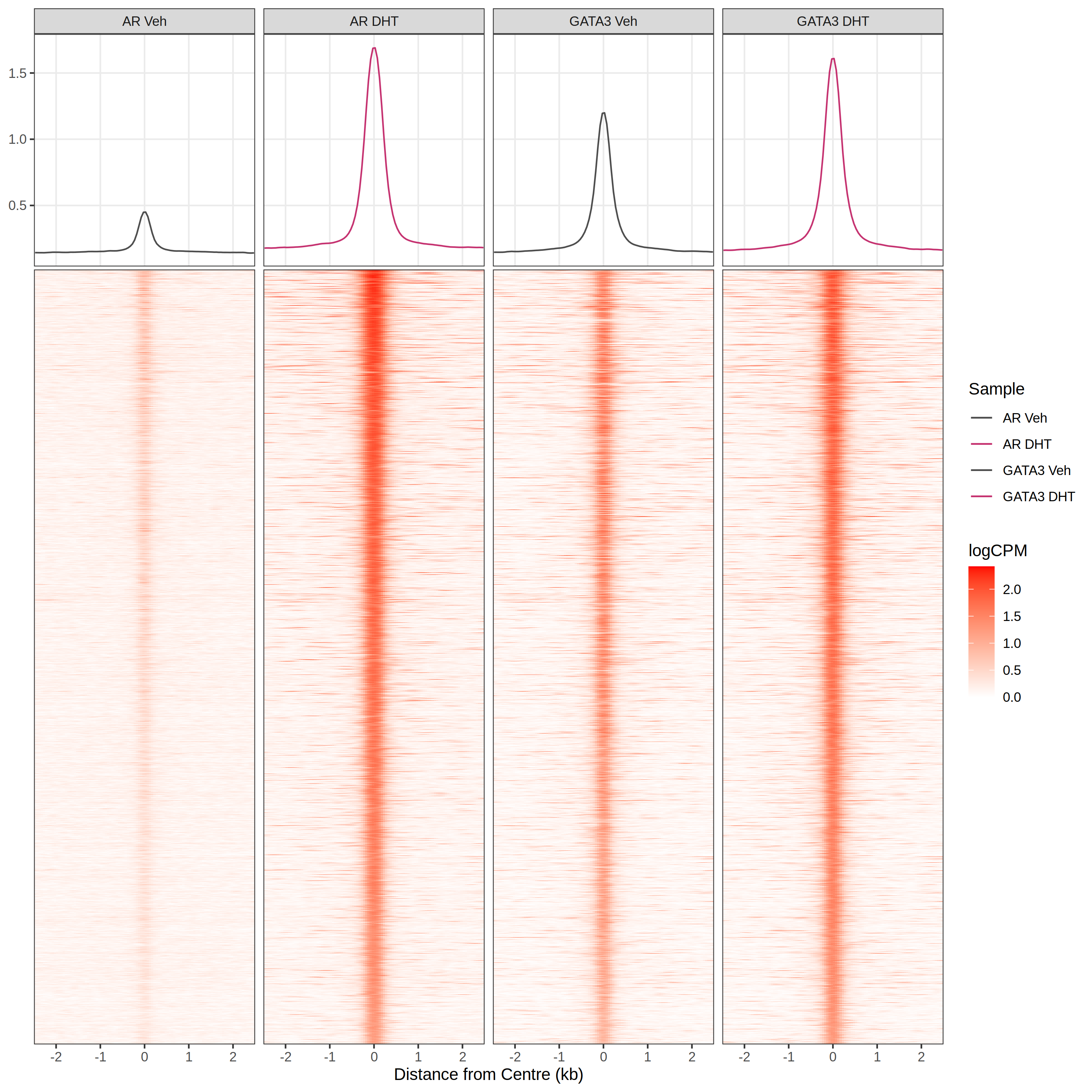
plotProfileHeatmap()
- Provide a set of ranges
- Centre & standardise width
- Read in data from
BigWigFileListgetProfileData(bwfl, gr)
- Plot data
- Uses
ggplot2for easy customisation- Top panel plots using
ggside
- Top panel plots using
- Still frustratingly slow… 😞
plotHFGC()
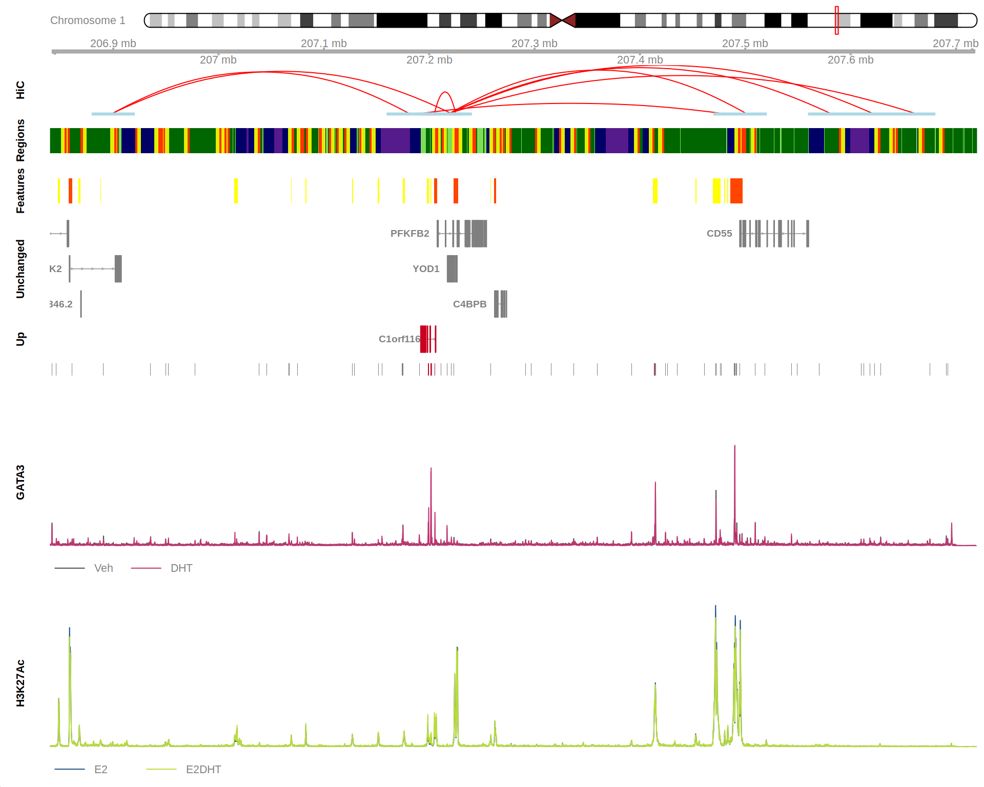
Here I’m checking binding for a DE gene (C1orf116)…
plotPie()
plotPie(consensus_peaks, fill = "region") +
  scale_fill_manual(values = colours$regions) +
  theme(legend.position = "none")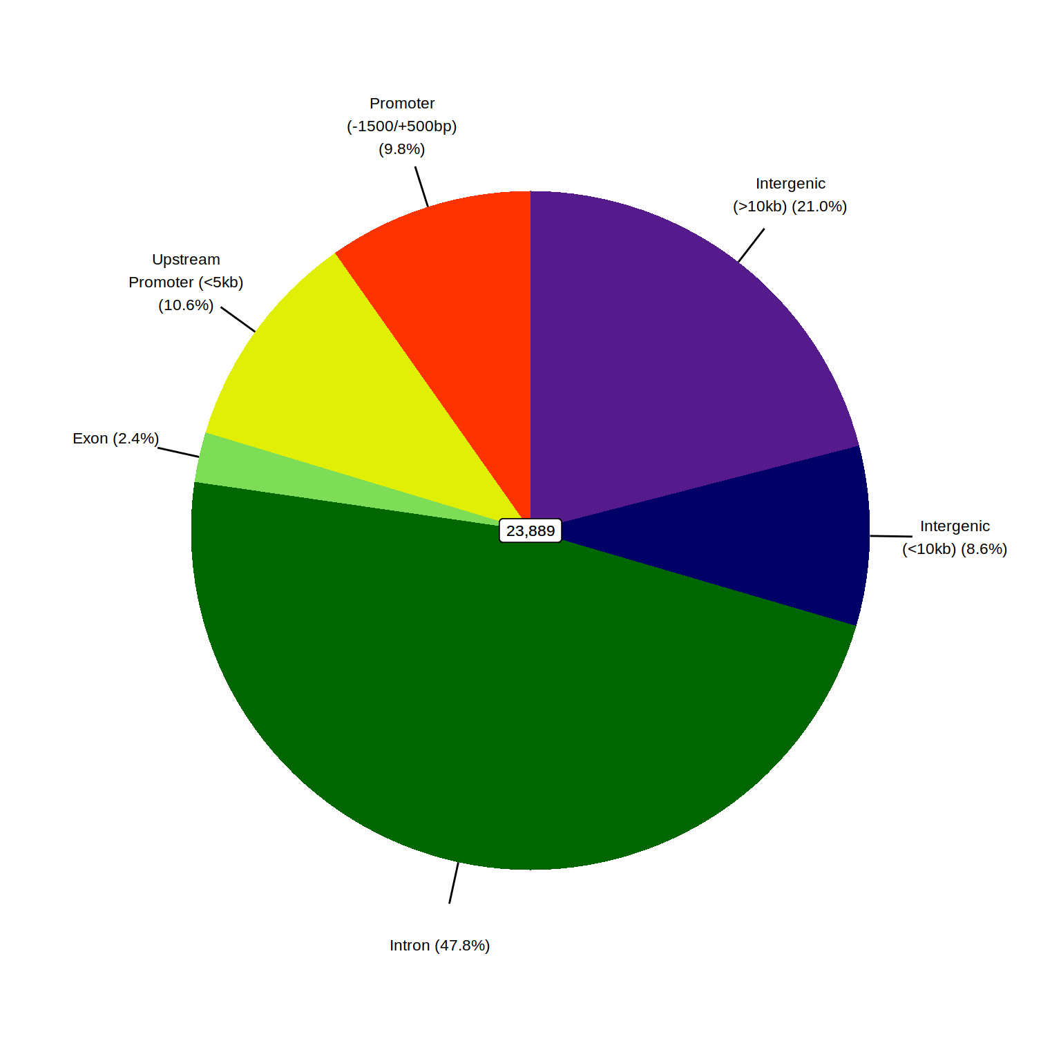
AR binding sites mapped to genomic regions
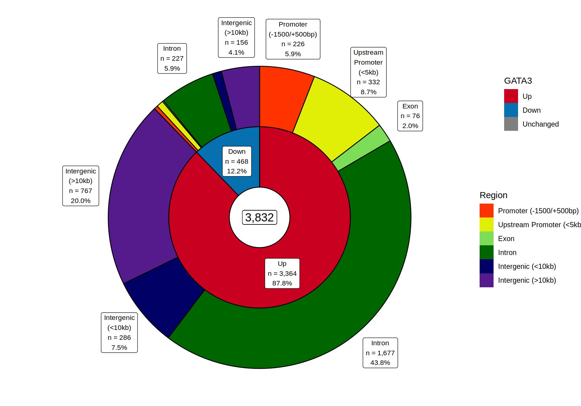
plotSplitDonut()
target <- "GATA3
merged_results %>%
  plotSplitDonut(
    inner = target, outer = "Region", min_p = 0.01,
    inner_glue = "{.data[[inner]]}\nn = {comma(n, 1)}\n{percent(p, 0.1)}",
    outer_glue = "{str_wrap(.data[[outer]], 12)}\nn = {comma(n, 1)}\n{percent(p, 0.1)}",
    inner_palette = direction_colours, outer_palette = region_colours
  )
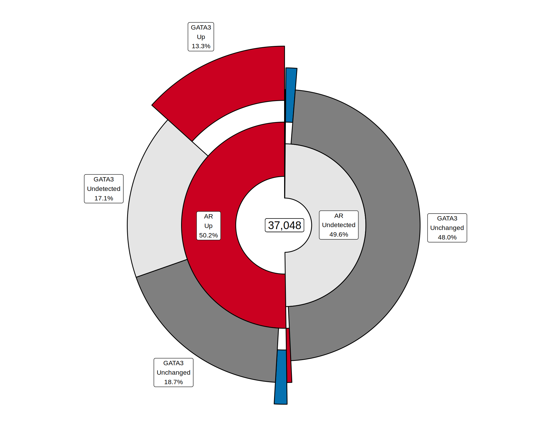
plotSplitDonut()
all_windows %>%
  plotSplitDonut(
    inner = colnames(.)[[1]], outer = colnames(.)[[2]], min_p =0.02,
    inner_glue = "{inner}\n{.data[[inner]]}\n{percent(p, 0.1)}",
    outer_glue = "{outer}\n{.data[[outer]]}\n{percent(p, 0.1)}",
    explode_inner = "Down|Up", explode_outer = "Down|Up", explode_r = 0.4,
    explode_query = "OR", nudge_r = 0.5,
    inner_palette = colours$direction, outer_palette = colours$direction
    inner_legend = FALSE, outer_legend = FALSE
) 
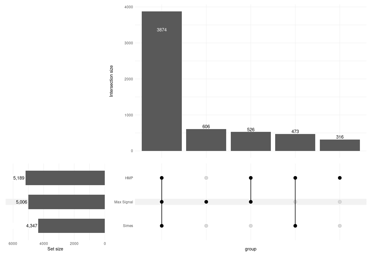
plotOverlaps()
- Calls 1)
ComplexUpset::upset()or 2)VennDiagram::draw.*wise.venn() - Size-scaled Venn Diagrams are tricky in
R…
ex <- list(x = letters[1:5], y = letters[c(6:15, 26)], z = letters[c(2, 10:25)])
plotOverlaps(ex, type = "upset", set_col = 1:3, labeller = stringr::str_to_title)
An Example
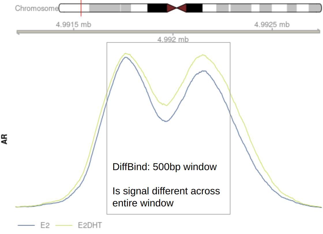
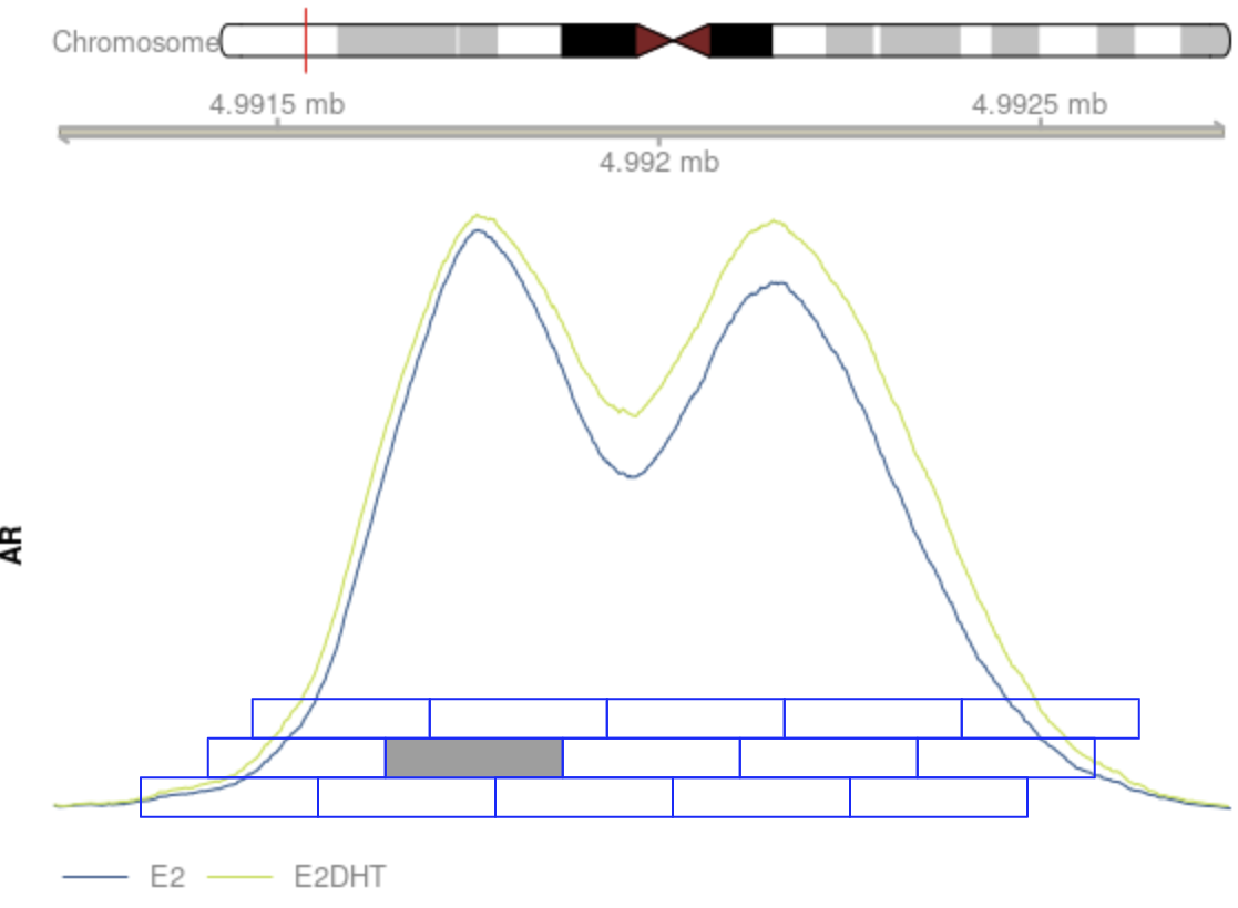
Use the maximal signal window?
extraChIPs: Window Merging
- Outperforms Simes’ consistently
Results Example 1
A ~3kb H3K27ac region unique to harmonic mean
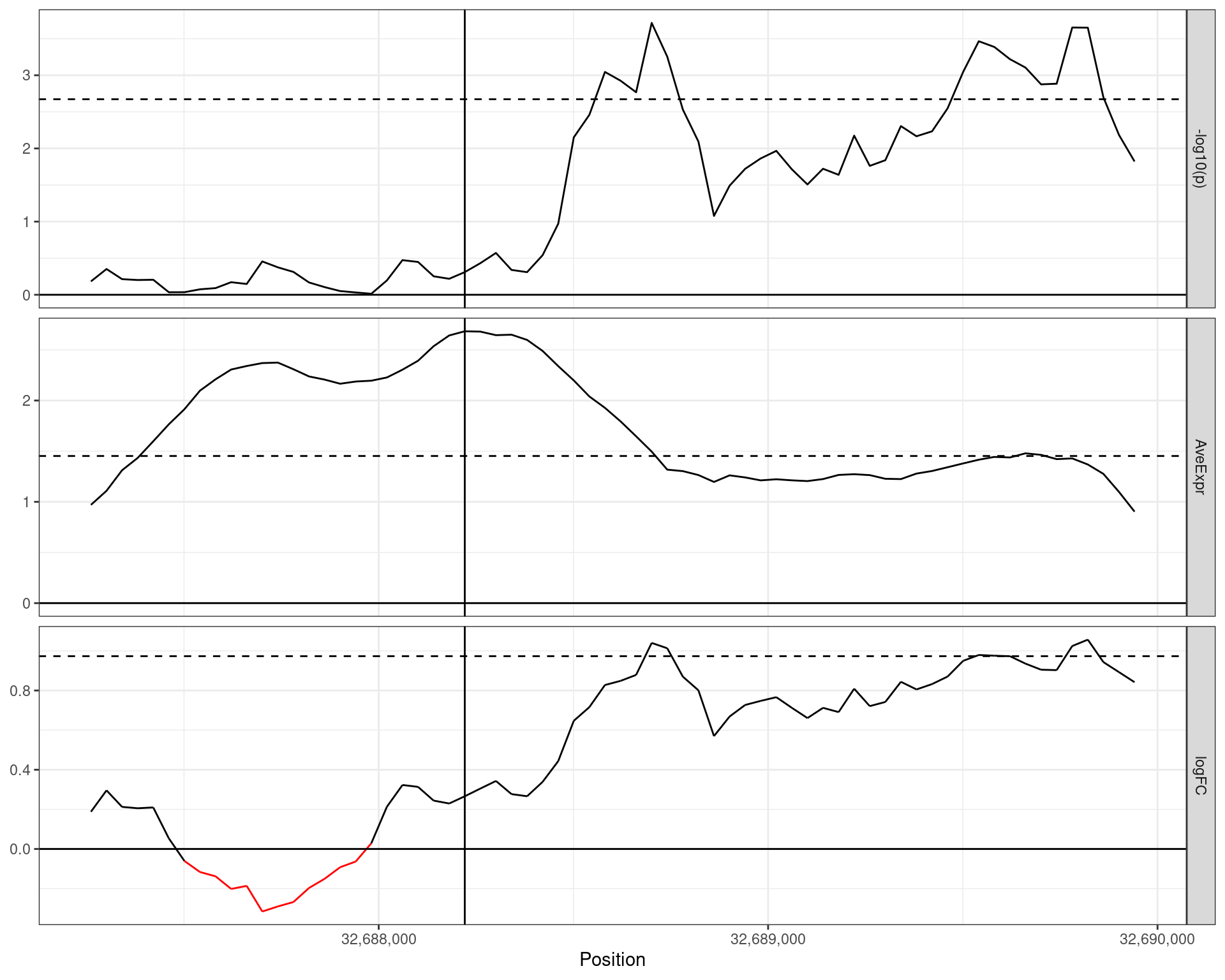
- \(-\log_{10}p\) in the top panel
- Dashed line is \(-\log_{10}(\text{hmp})\)
- Dashed line is \(-\log_{10}(\text{hmp})\)
- Average Signal is the middle panel
- Dashed line is weighted mean
- Dashed line is weighted mean
- logFC in bottom panel
- Dashed line is weighted mean
- Vertical line is maximal signal
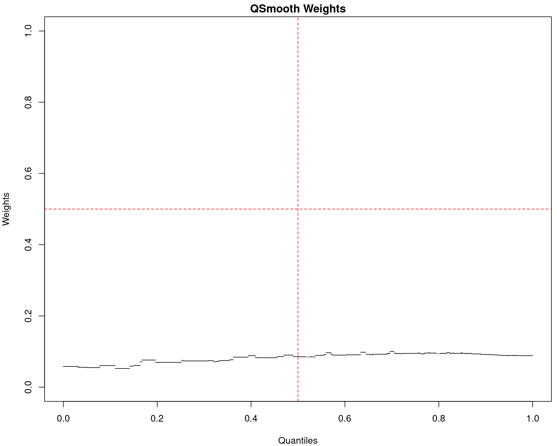
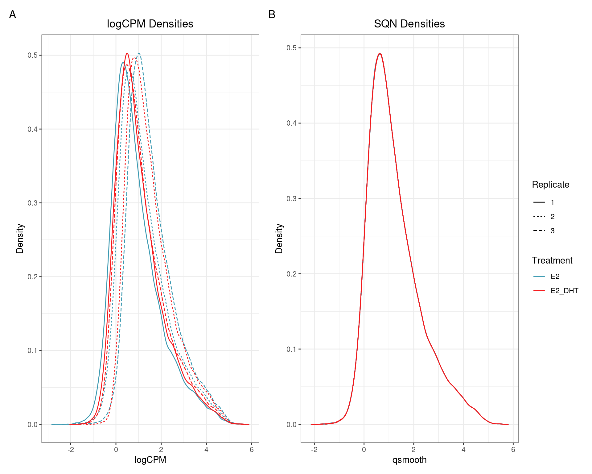
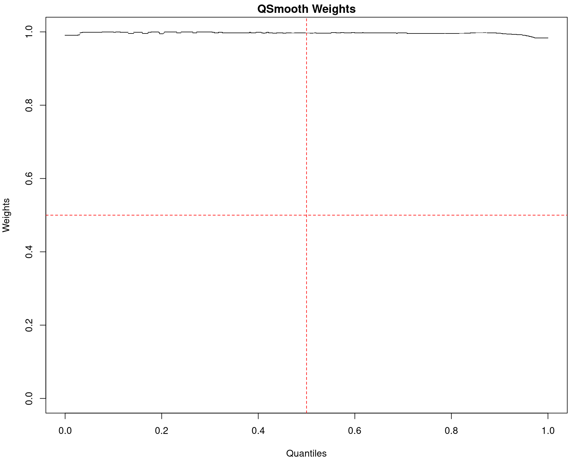
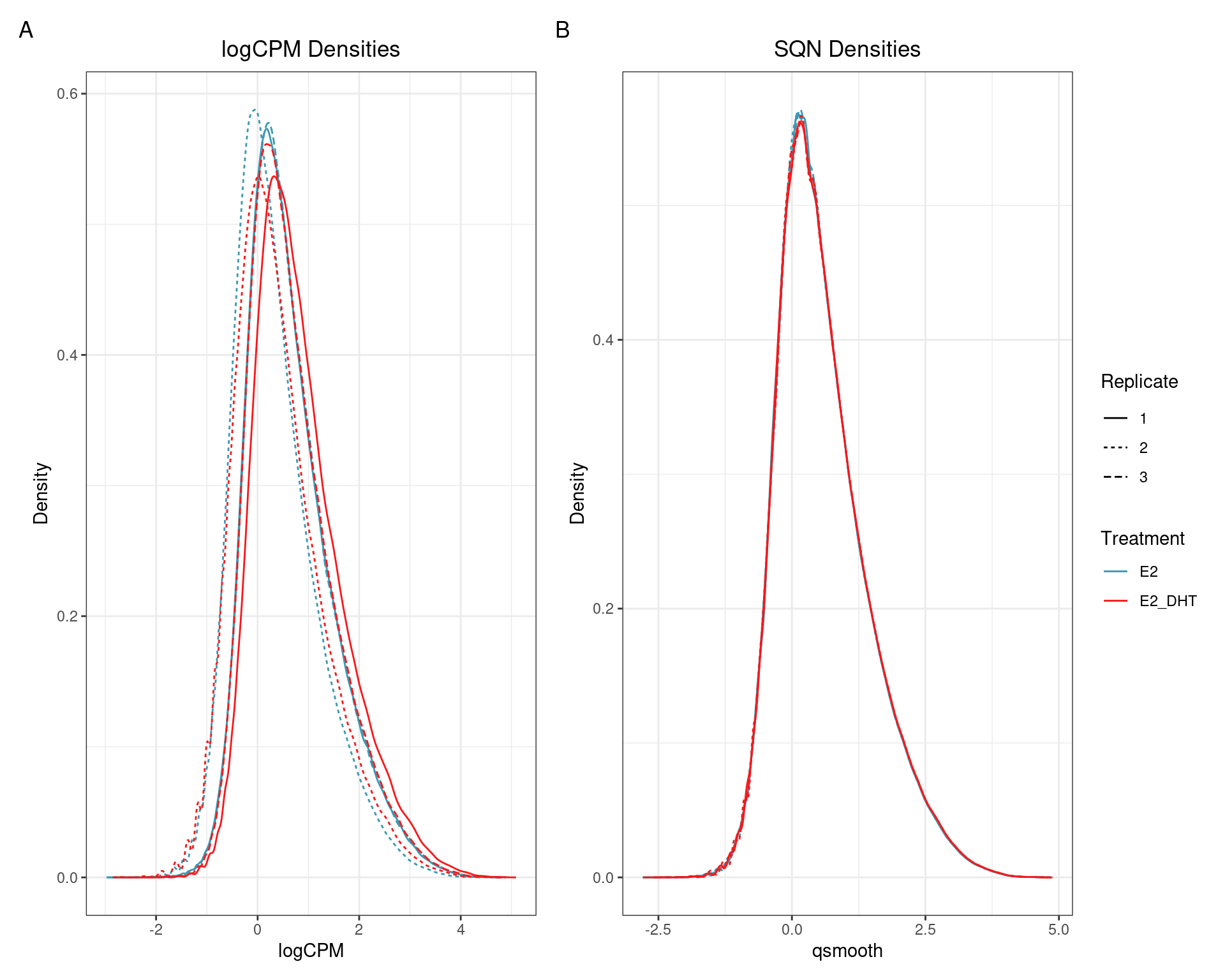
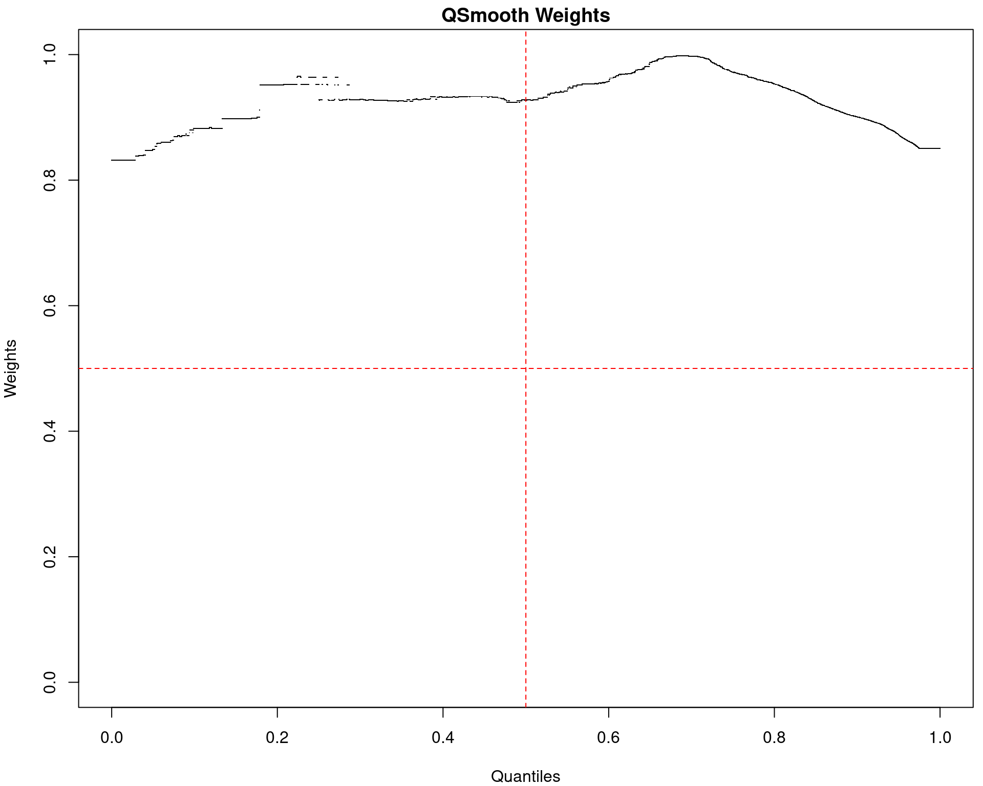
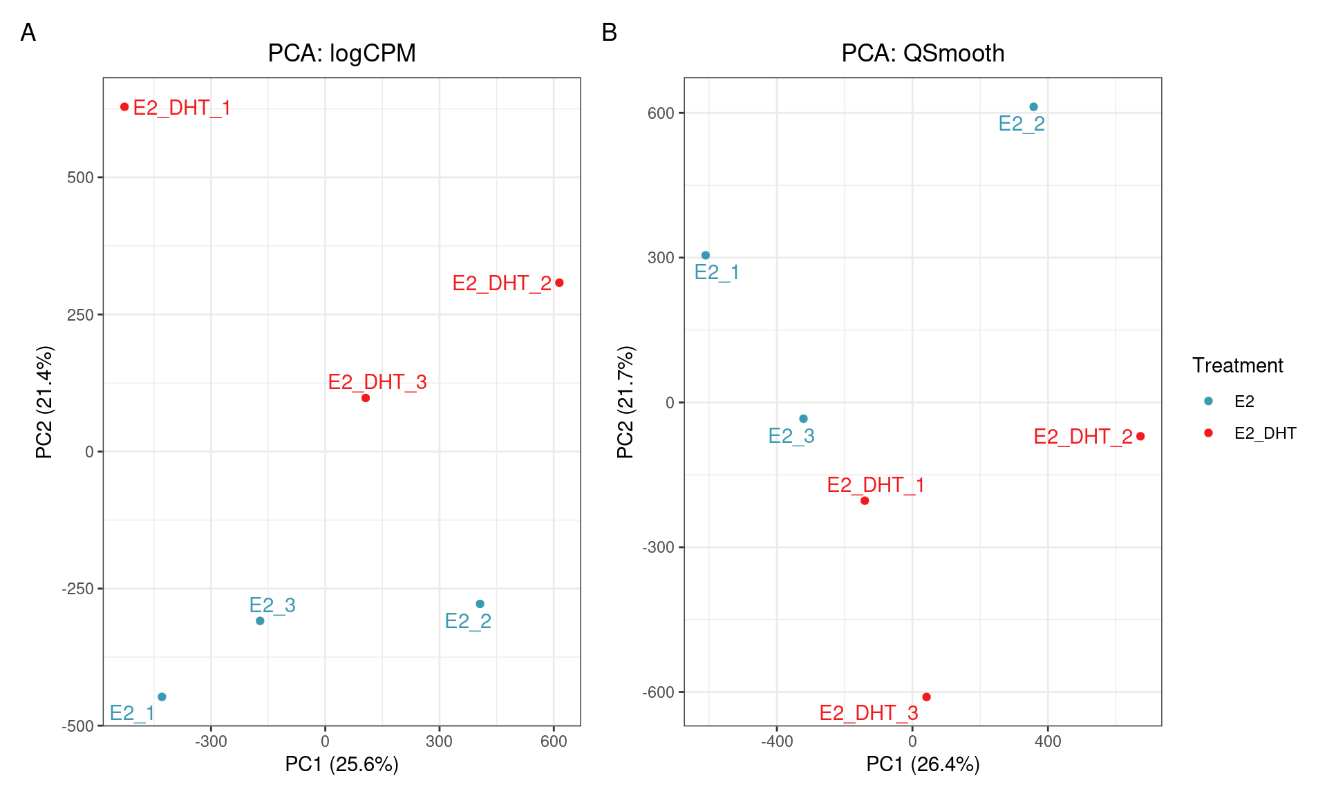
SQN
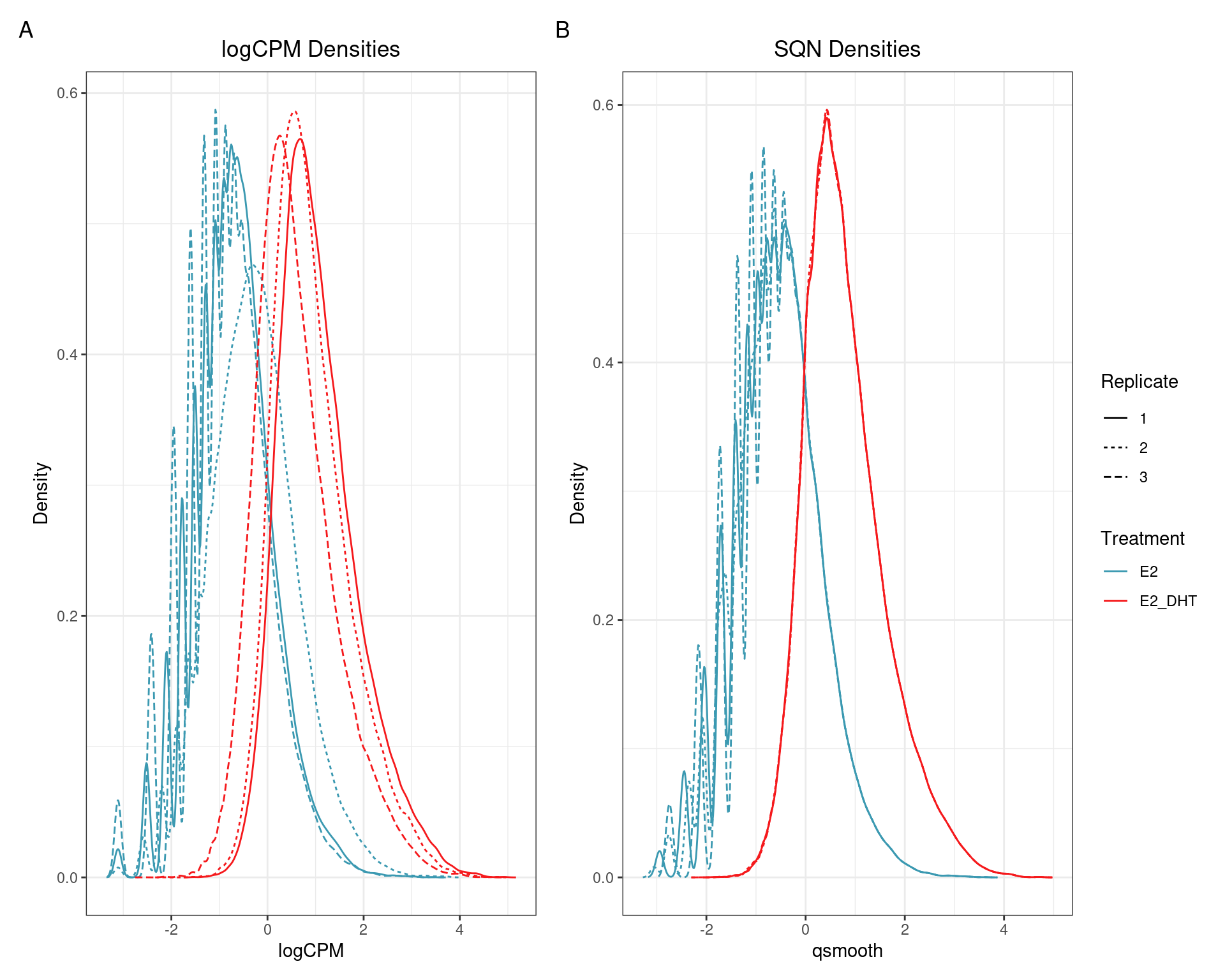
(quantro: \(p_{med} = 0.002\); \(p_{dist} < 5e4\))
(quantro: \(p_{med} = 0.91\); \(p_{dist} = 0.42\))
(quantro: \(p_{med} = 0.65\); \(p_{dist} < 5e4\))
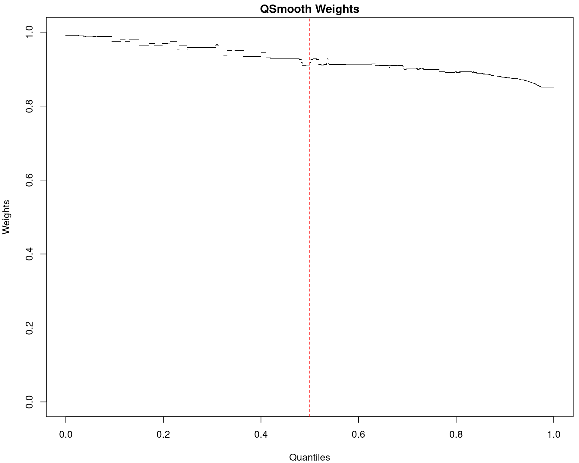
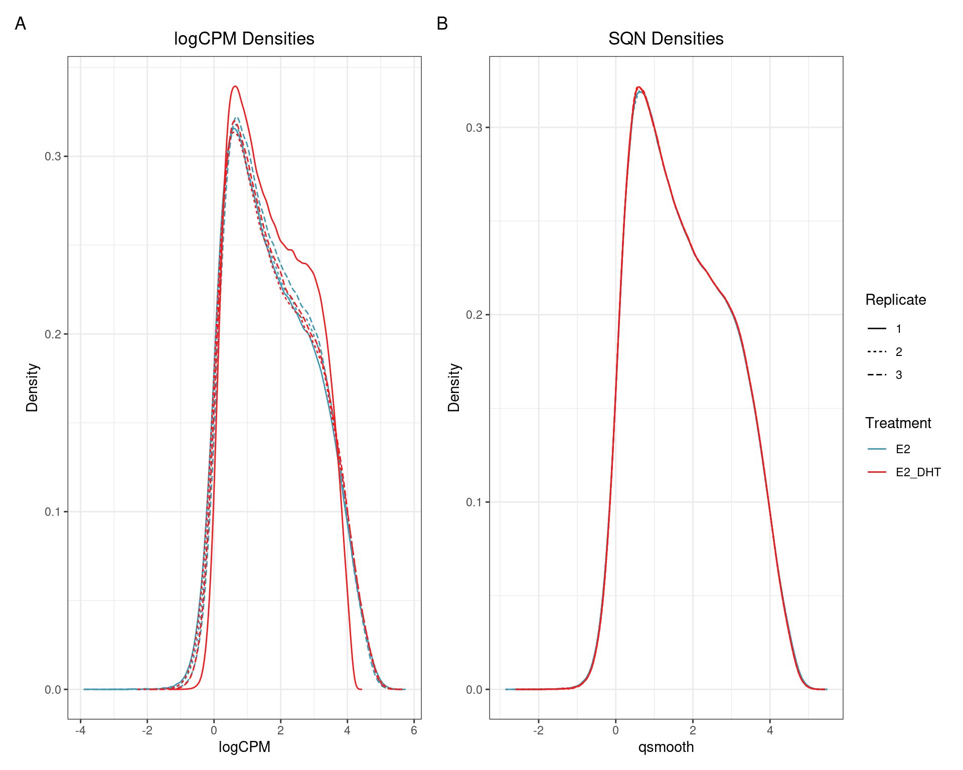
(quantro: \(p_{med} = 0.84\); \(p_{dist} = 0.49\))
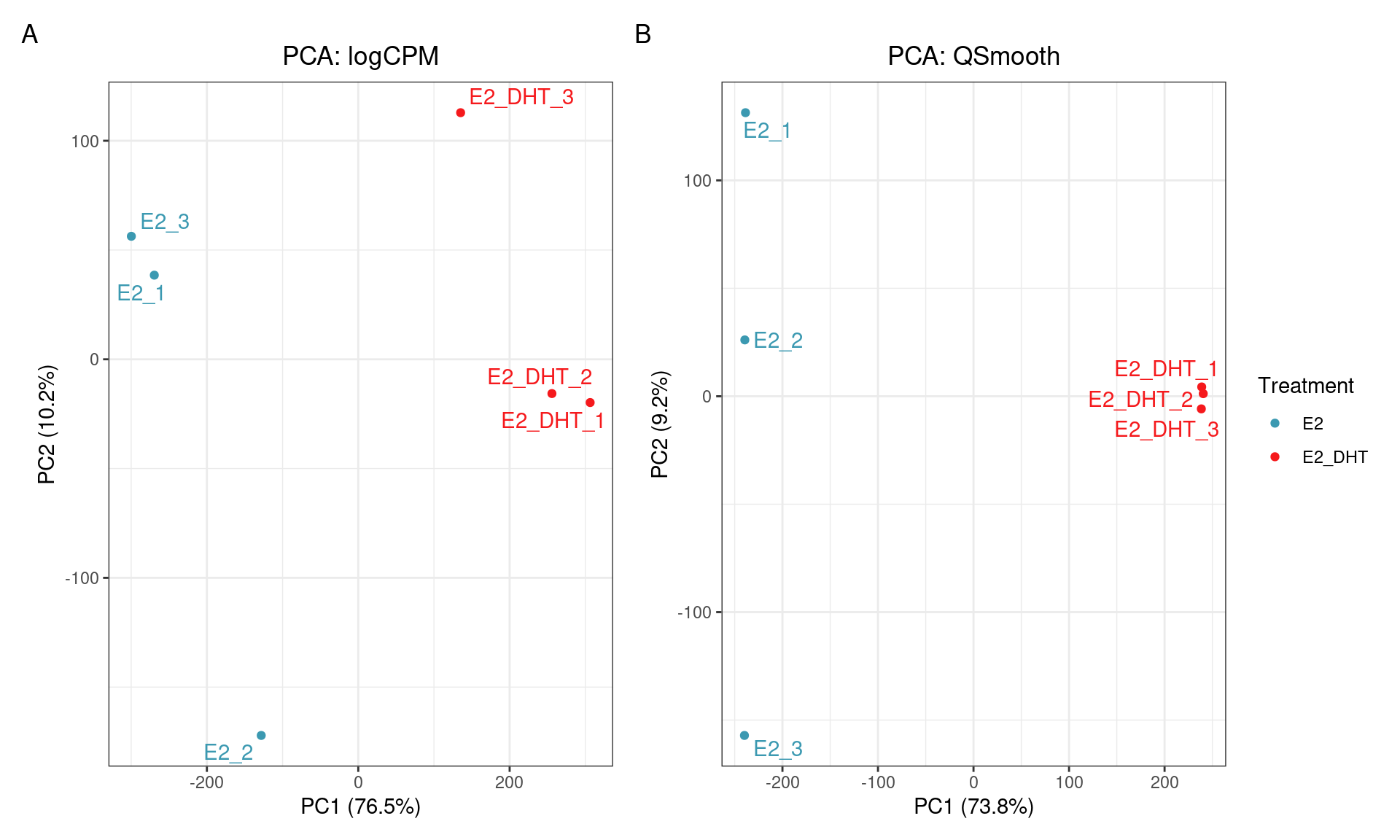
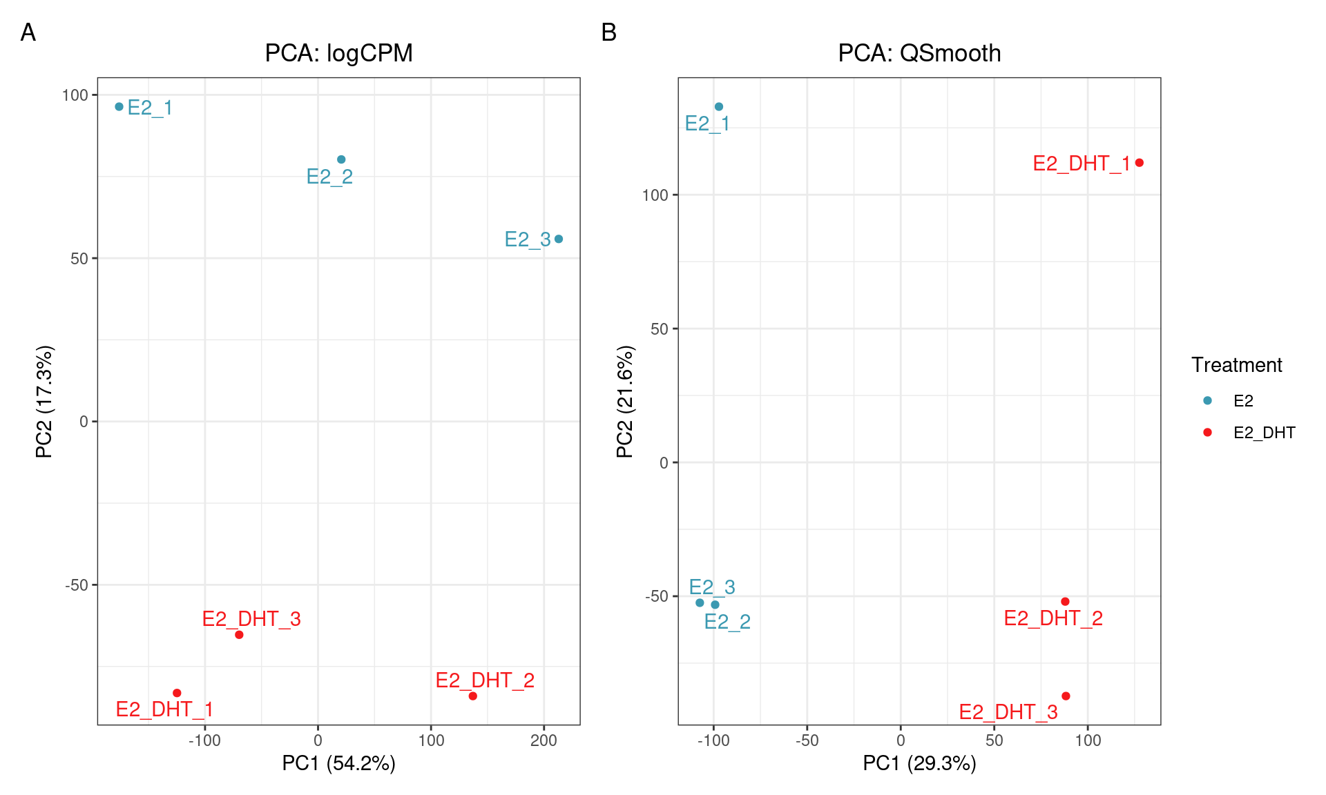
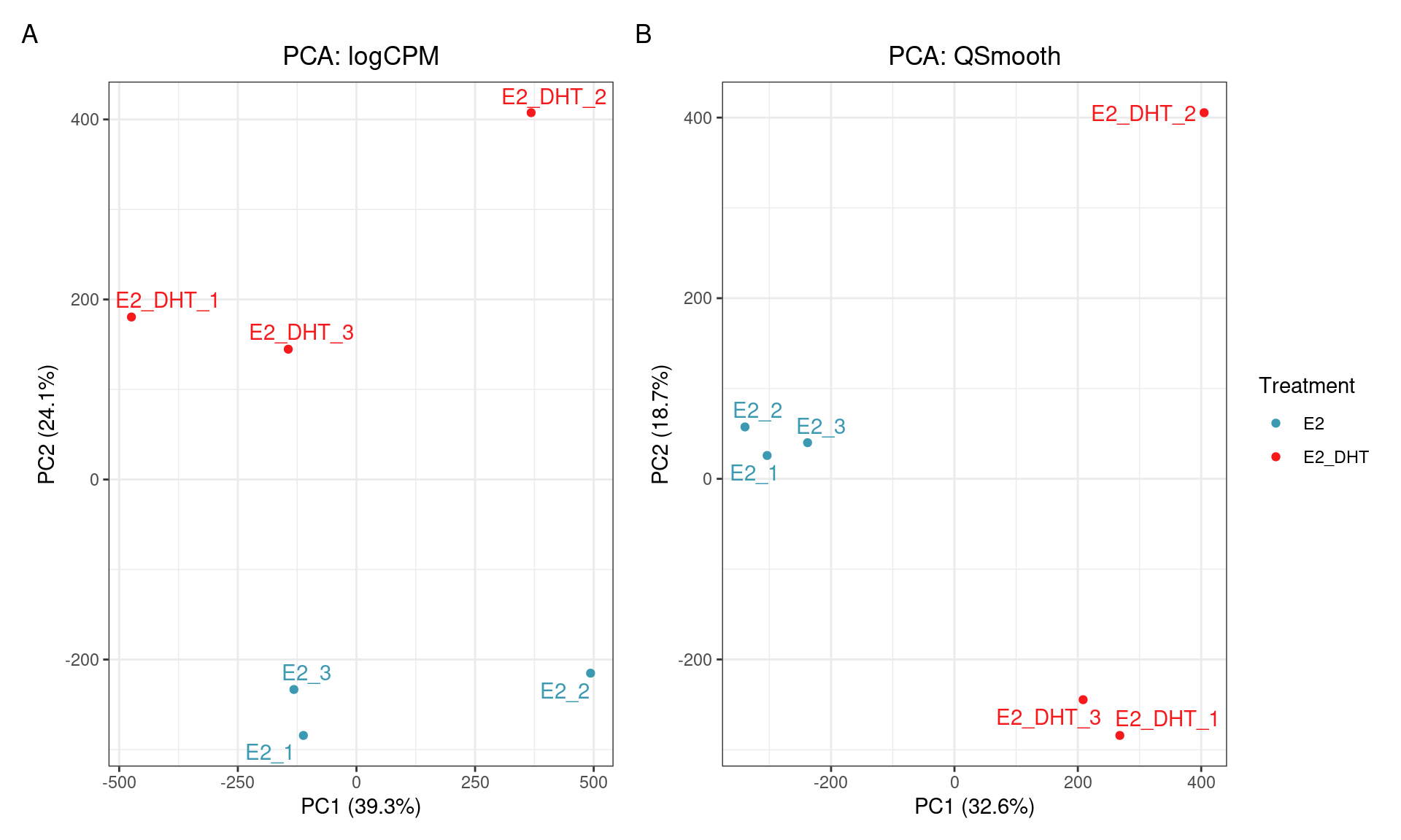
SQN: PCA
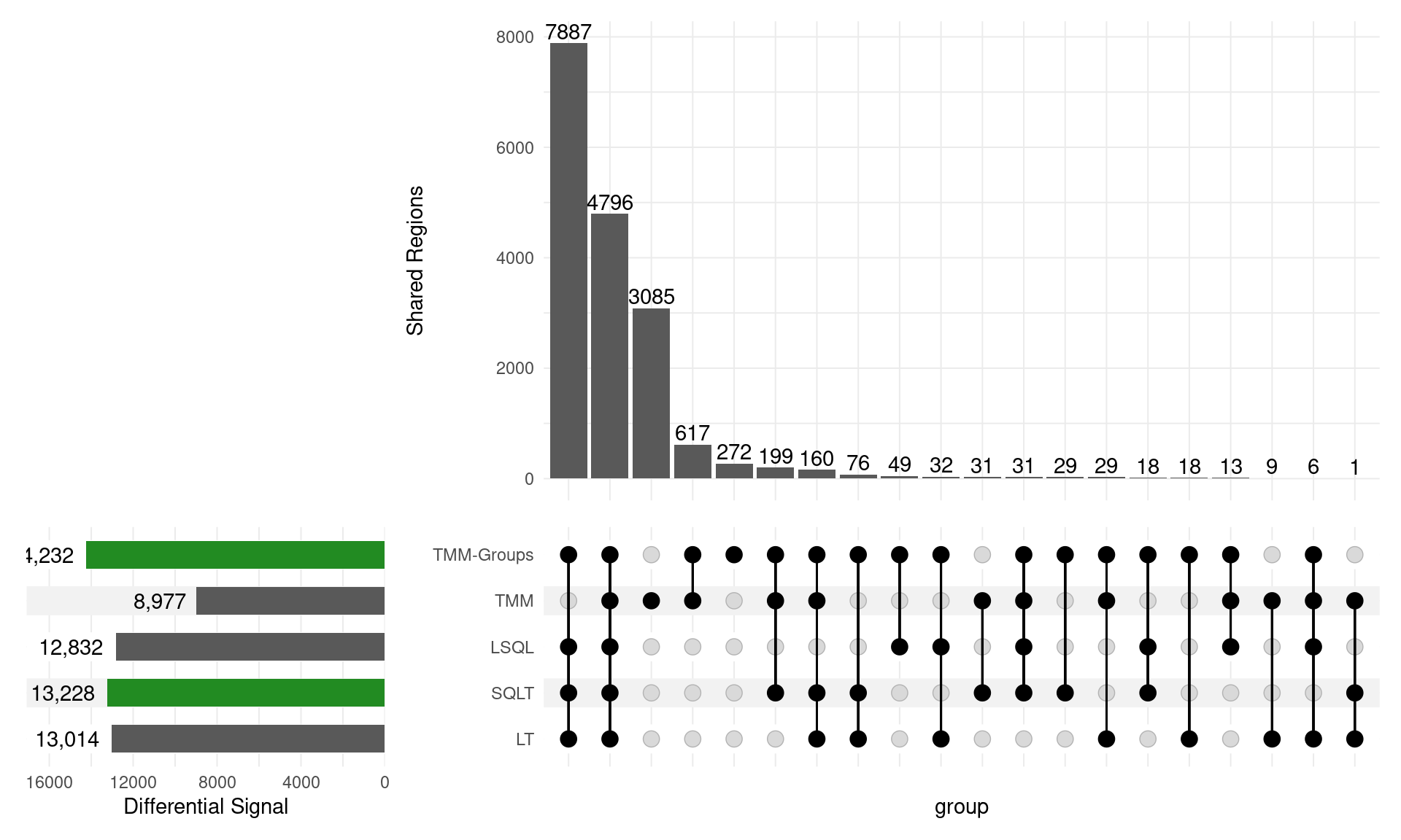
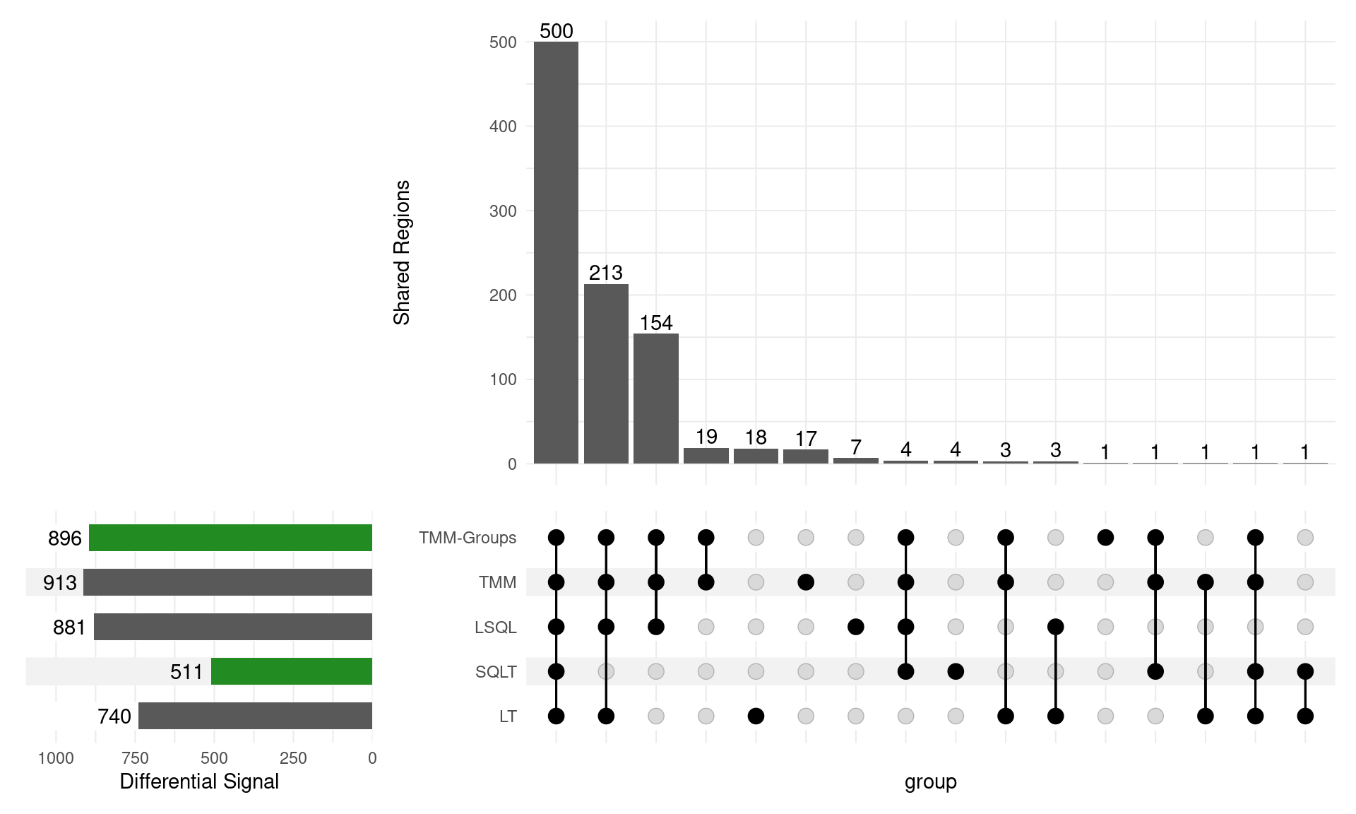
Overall Results
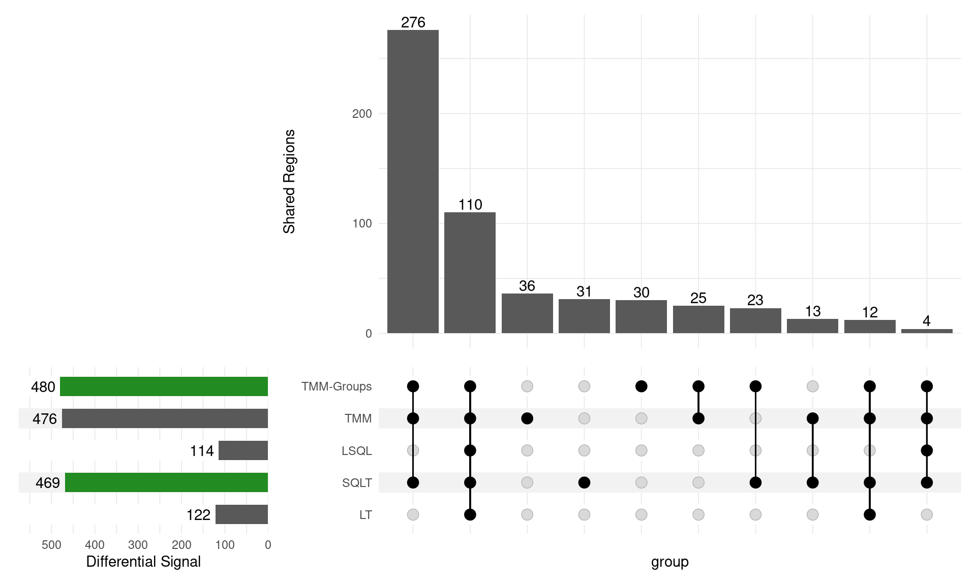
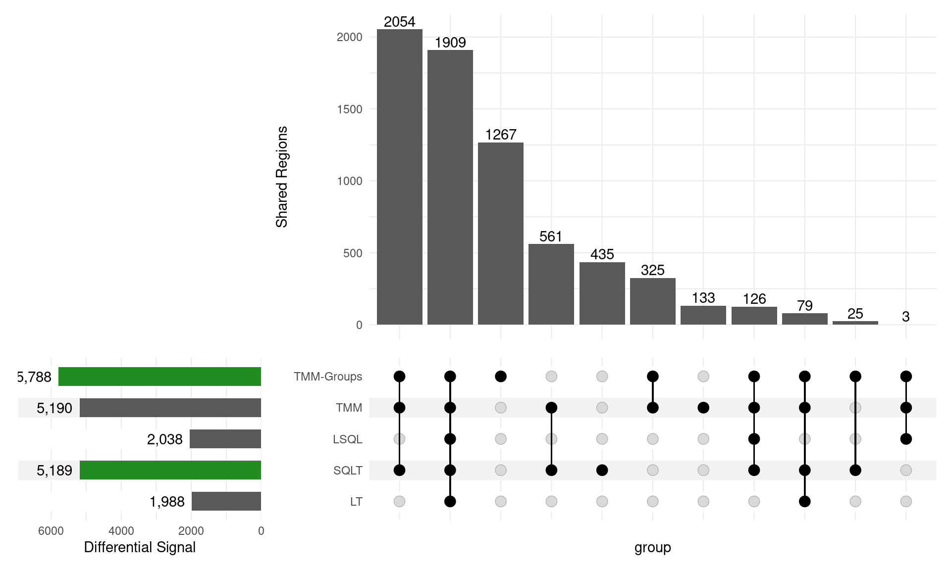
Directional Results
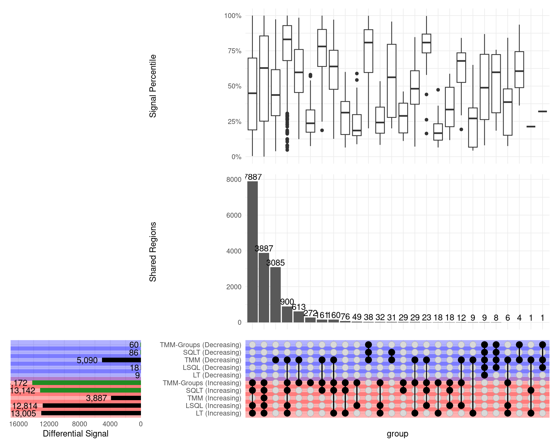
GATA3
\(H_0\): logFC = 0
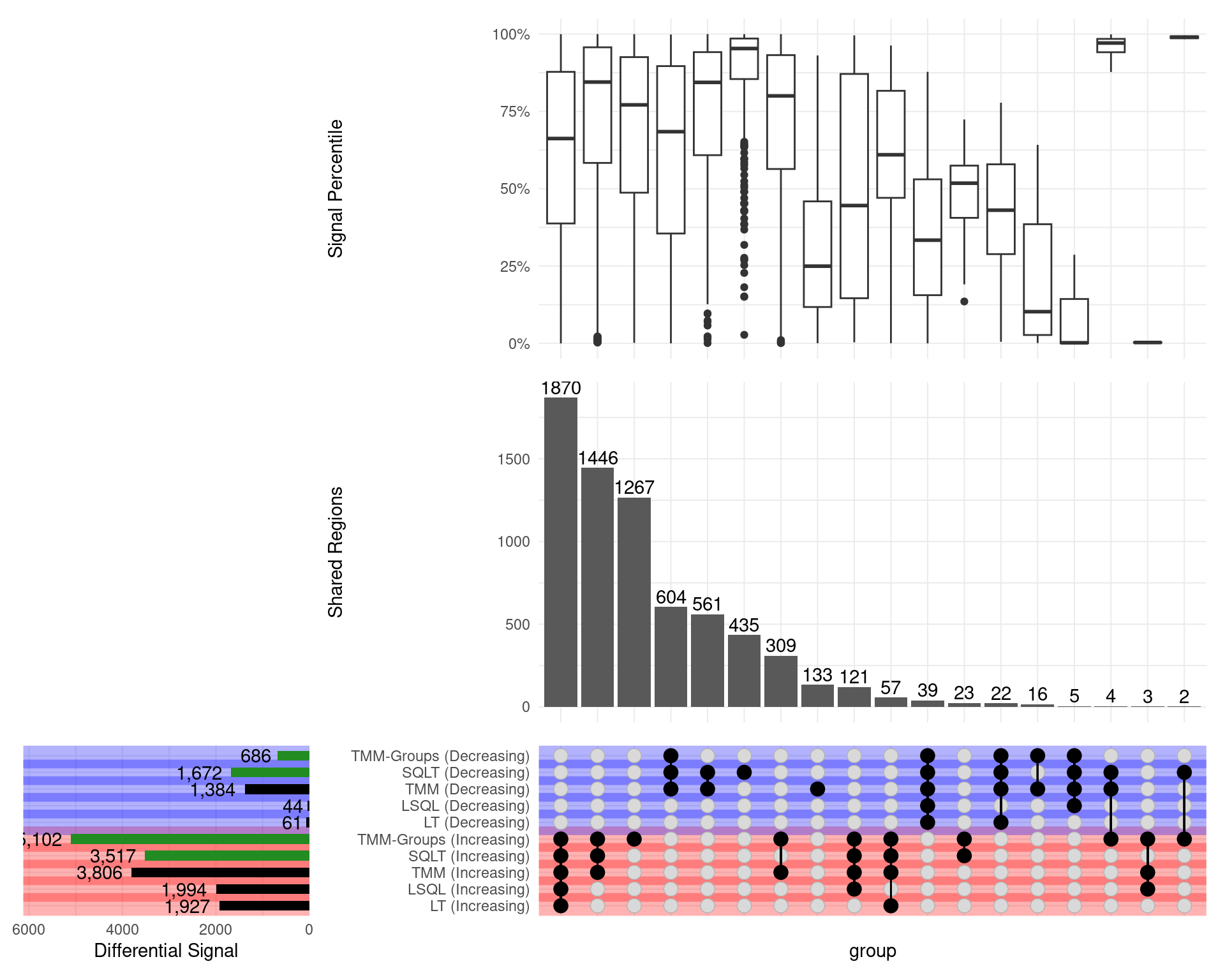
- SQLT has the most decreasing sites
- Less competitive for increasing
GATA3
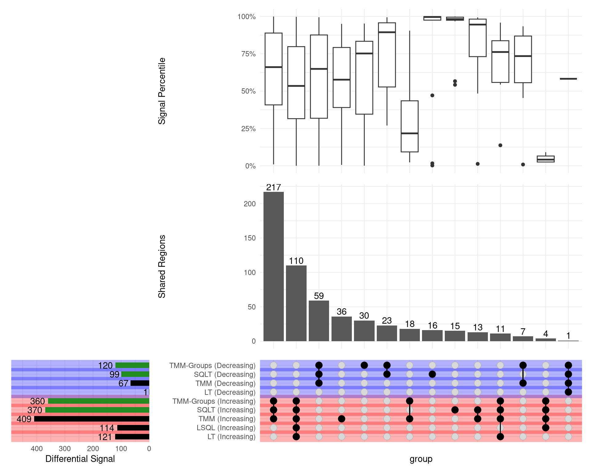
Range-based \(H_0\)
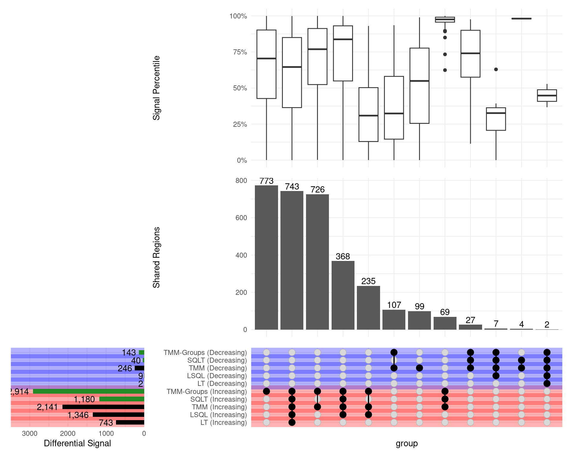
- SQLT now has only 40 down sites (from 1672)
- TMM Groups only dropped from 686 to 143
MA Plots: GATA3
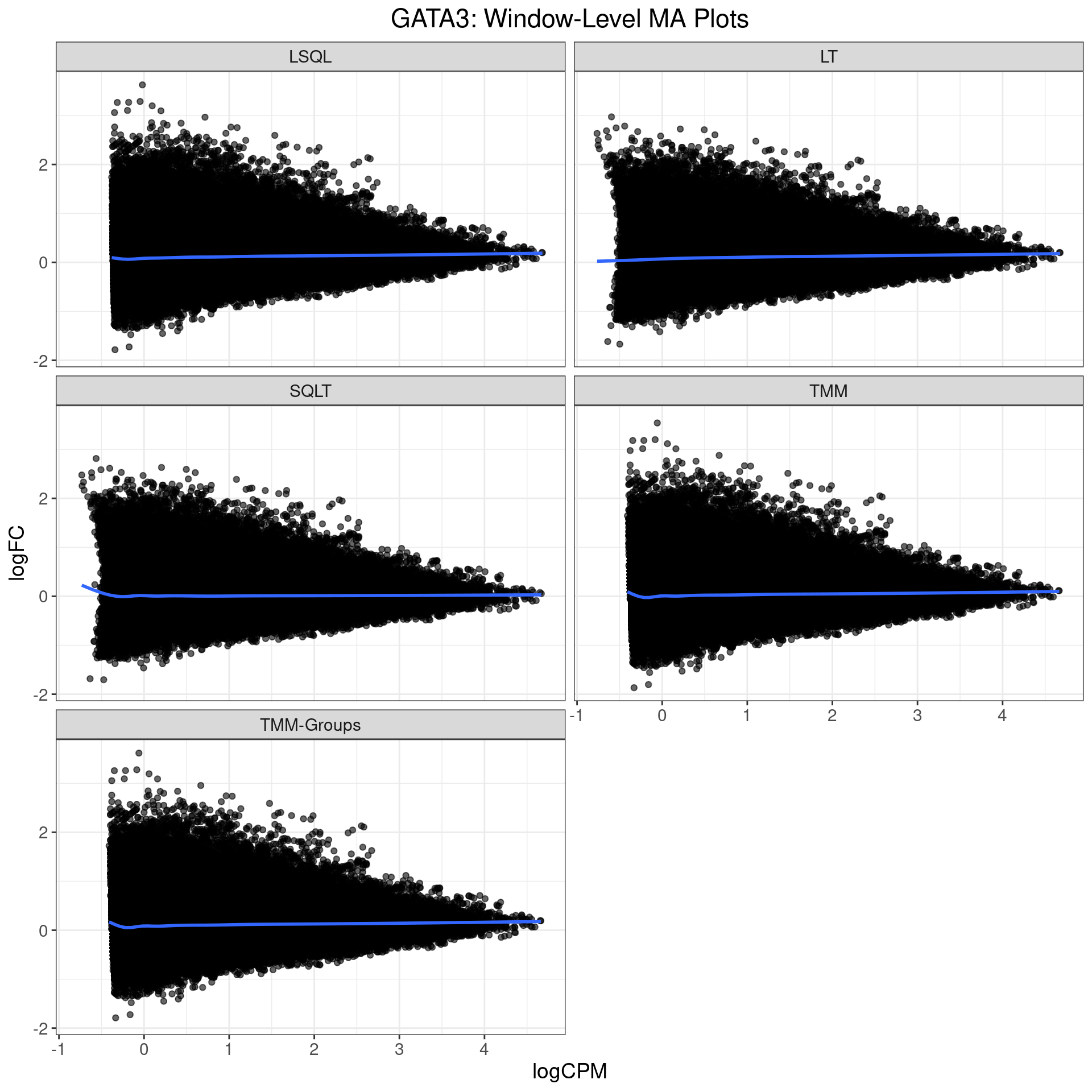
- Small positive bias in Library Size only (LSQL & LT)
- Small positive bias in TMM & TMM-Groups
- Is this why more gained sites?
- No apparent bias in SQLT
- Is ‘under-performance’ actually good?
- SQLT also appears more range-restricted
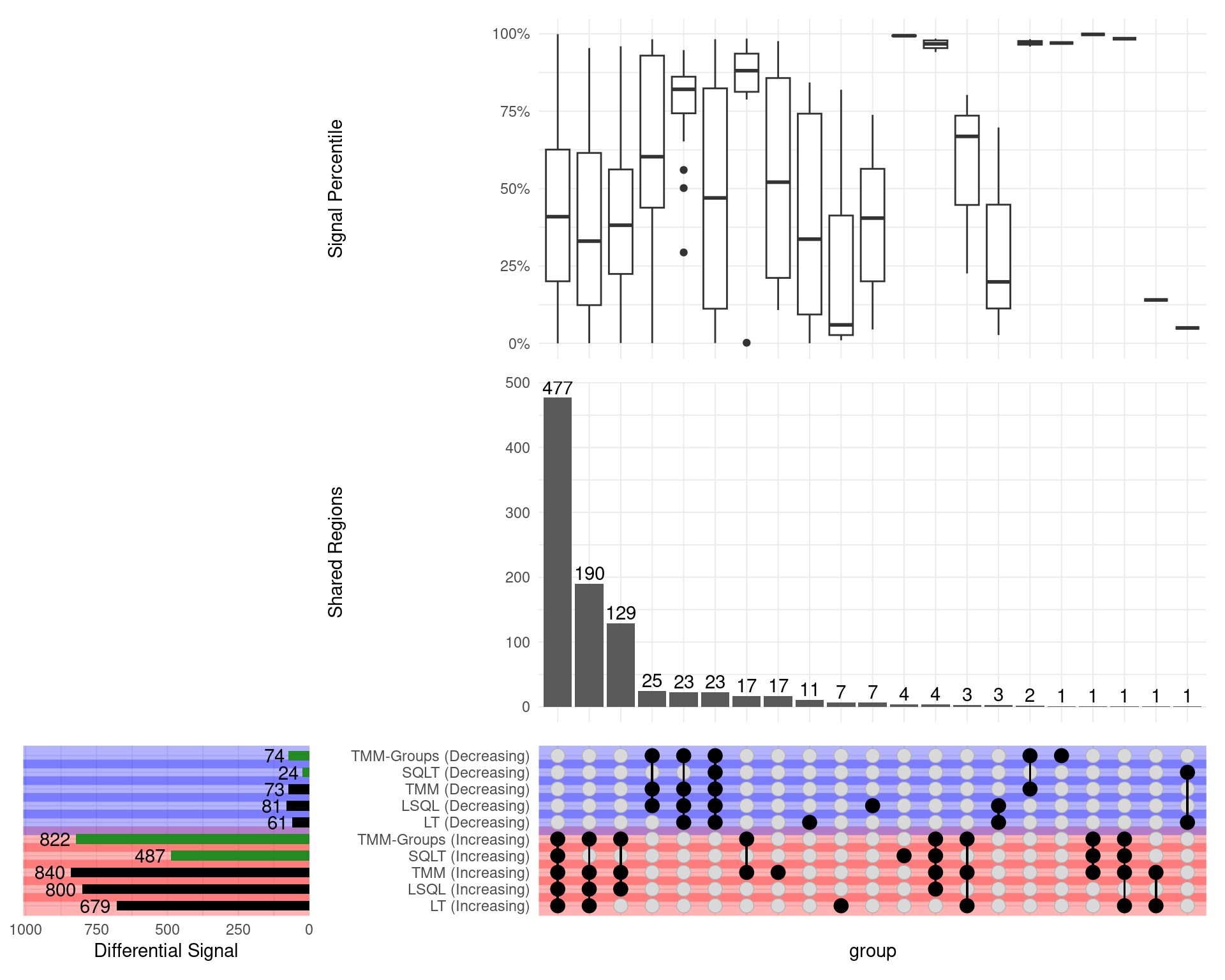
MA Plots: H3K27ac
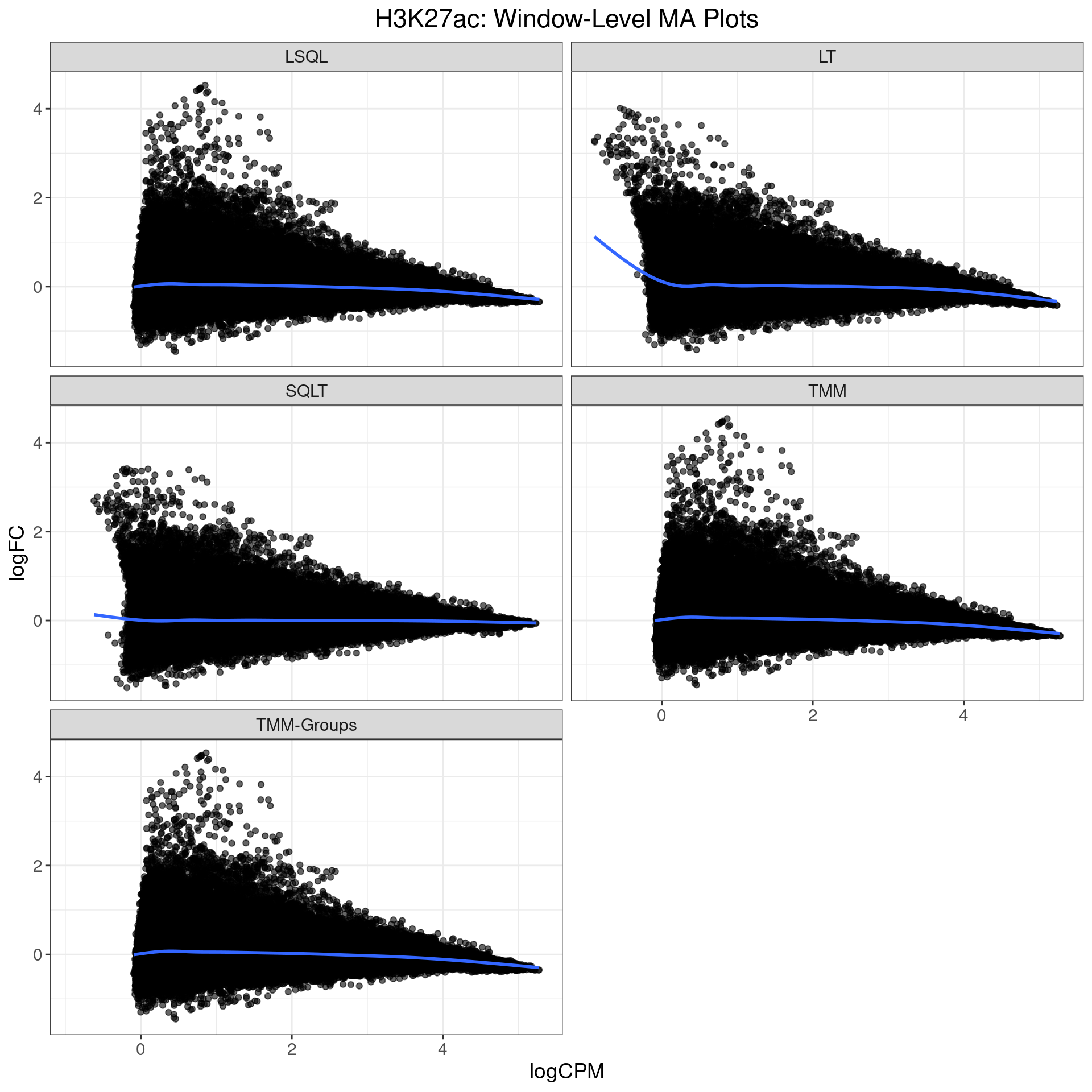
- Bias in all methods bar SQLT
- Most likely due to outlier sample
- Doesn’t quite explain the results
- Difference was mainly in Gains
logFC Comparison: LSQL Vs LT
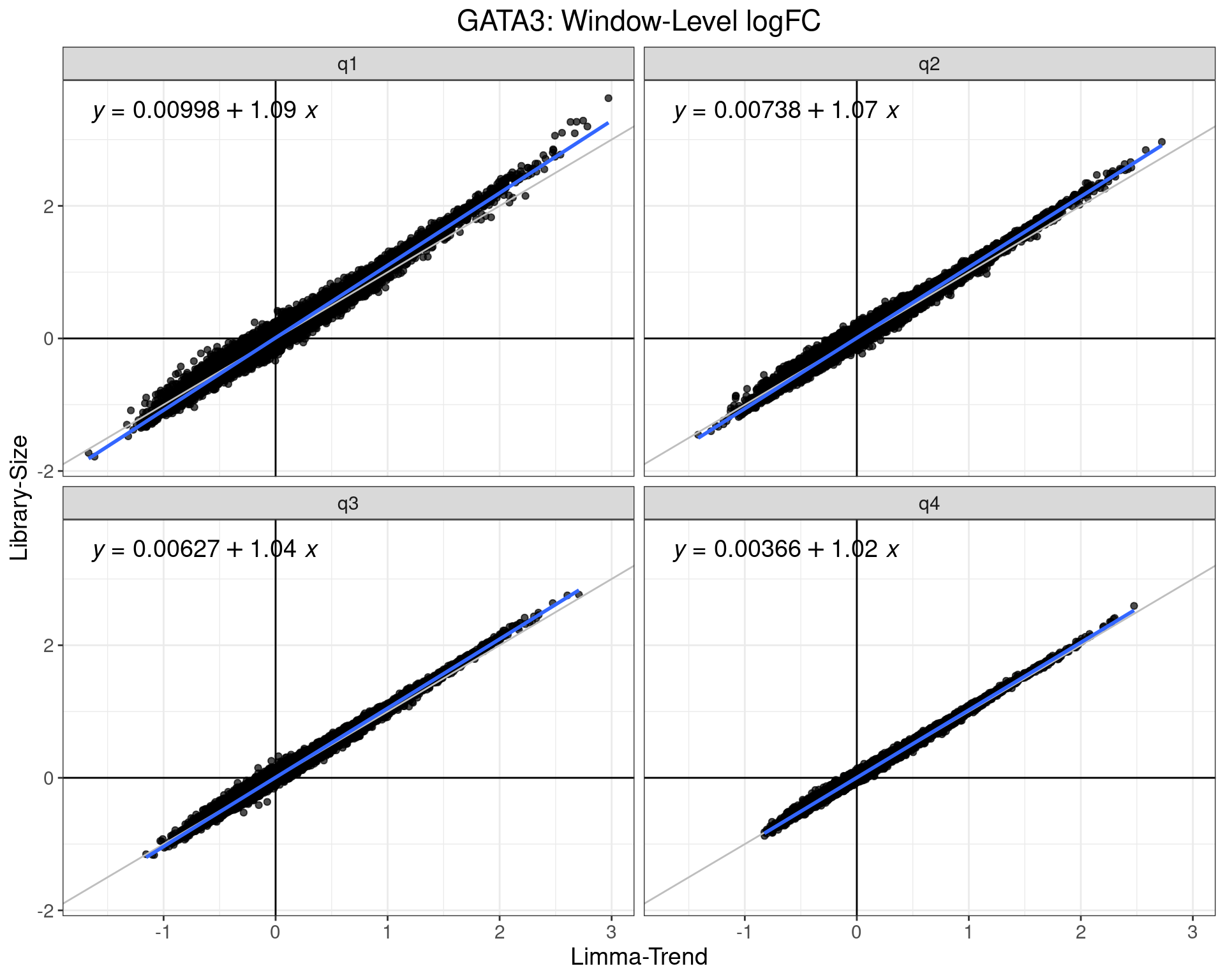
- Estimates from GLM-QL model are consistently higher
- Far more so in the lowest signal quartile
- Similar patterns in most datasets
logFC Comparison: SQLT Vs TMM-Groups
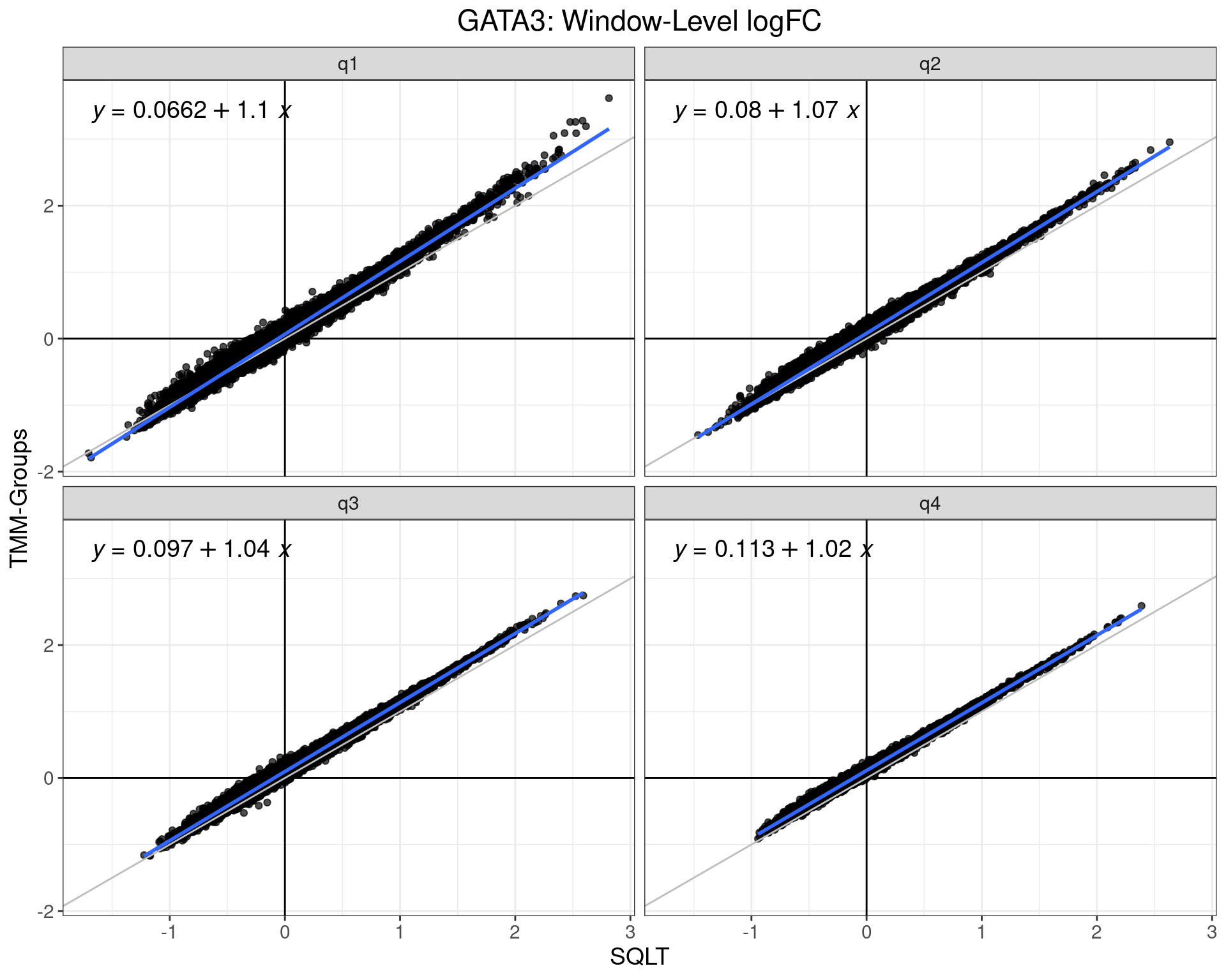
- Effect is even more pronounced for estimates using within-group normalisation
- Do I need to change the
treatthreshold?- Does GLM-20% = SQLT-18% in high quartile
- Does GLM-20% = SQLT-10% in the low quartile?
References
Hickey, Theresa E, Luke A Selth, Kee Ming Chia, Geraldine Laven-Law, Heloisa H Milioli, Daniel Roden, Shalini Jindal, et al. 2021. “The Androgen Receptor Is a Tumor Suppressor in Estrogen Receptor-Positive Breast Cancer.” Nat. Med. 27 (2): 310–20.
Hicks, Stephanie C, and Rafael A Irizarry. 2015. “Quantro: A Data-Driven Approach to Guide the Choice of an Appropriate Normalization Method.” Genome Biol. 16 (1): 117.
Hicks, Stephanie C., Kwame Okrah, Joseph N. Paulson, John Quackenbush, Rafael A. Irizarry, and Hector Corrado Bravo. 2018. “Smooth Quantile Normalization.” Biostatistics 19 (2).
Law, Charity W, Yunshun Chen, Wei Shi, and Gordon K Smyth. 2014. “Voom: Precision Weights Unlock Linear Model Analysis Tools for RNA-seq Read Counts.” Genome Biol. 15 (2): R29.
Lun, Aaron T L, and Gordon K Smyth. 2014. “De Novo Detection of Differentially Bound Regions for ChIP-Seq Data Using Peaks and Windows: Controlling Error Rates Correctly.” Nucleic Acids Res. 42 (11): e95.
———. 2016. “Csaw: A Bioconductor Package for Differential Binding Analysis of ChIP-Seq Data Using Sliding Windows.” Nucleic Acids Res. 44 (5): e45.
McCarthy, Davis J, and Gordon K Smyth. 2009. “Testing Significance Relative to a Fold-Change Threshold Is a TREAT.” Bioinformatics 25 (6): 765–71.
Ross-Innes, Caryn S., Rory Stark, Andrew E. Teschendorff, Kelly A. Holmes, H. Raza Ali, Mark J. Dunning, Gordon D. Brown, et al. 2012. “Differential Oestrogen Receptor Binding Is Associated with Clinical Outcome in Breast Cancer.” Nature 481: –4. http://www.nature.com/nature/journal/v481/n7381/full/nature10730.html.
Wilson, Daniel J. 2019. “The Harmonic Mean p-Value for Combining Dependent Tests.” Proc. Natl. Acad. Sci. U. S. A. 116 (4): 1195–1200.