Using extraChIPs with GRAVI

Hot mess or slick analysis?

Stephen (Stevie) Pederson

BiocAsia

2022-12-01

Introduction

Who Am I?

Post-doctoral Bioinformatician (ECR)
- Black Ochre Data Laboratories
- Based in Adelaide, South Australia
- Traditional lands of the Kaurna people

Author/Maintainer of ngsReports
- Parse & plot FastQC, cutadapt, STAR, macs2 etc.

GRAVI

2020 - 2022: Dame Roma Mitchell Cancer Research Laboratories (DRMCRL)
Activation of the Androgen Receptor (AR) as a therapeutic strategy for Breast Cancer (Hickey et al. 2021)
Combined genomic changes to AR, ER & GATA3 binding after DHT-treatment (ChIP-Seq)
- 4 cell lines + 2 PDX model
- Additional Histone Marks
- Additional HiC / HiChIP Data (Sometimes)
- RNA Seq data

GRAVI

Gene Regulatory Analysis using Variable Inputs (https://github.com/steveped/GRAVI)
snakemake workflow
- HTML Output inspired by workflowr (Blischak, Carbonetto, and Stephens 2019)
- All code visible \(\implies\) Reproducible as complete or in sections
- Standardised all output formats/structures

GRAVI

Minimal Data:
- 1 ChIP Target across two conditions
Best for 2-3 ChIP targets with 2-3 conditions
- Enables Pair-wise Comparisons
- Optional Data: RNA-Seq Results, HiC Interactions, Genomic Features (H3K27ac)

extraChIPs

GRAVI

extraChIPs was developed as key infrastructure for GRAVI
3 Primary sets of Functions
1. Working with GRanges focussed on mcols()
2. ChIP-Seq Helper Functions (i.e. peaks and differential binding)
3. Data Visualisation

Working With Ranges: `tibble` Coercion

## S3 method for class 'DataFrame'
as_tibble(x, rangeAsChar = TRUE, ...)

## S3 method for class 'GenomicRanges'
as_tibble(x, rangeAsChar = TRUE, name = "range", ...)

## S3 method for class 'Seqinfo'
as_tibble(x, ...)

## S3 method for class 'GInteractions'
as_tibble(x, rangeAsChar = TRUE, suffix = c(".x", ".y"), ...)

Defined for GRanges, DataFrame, Seqinfo and GInteractions classes
Handles S4 Compressed list columns well (so far)
- Uses vctrs::vec_proxy() to coerce to S3 lists

Working With Ranges: `tibble` Coercion

Starting with the protein-coding transcripts for CTLA4

gr

GRanges object with 4 ranges and 2 metadata columns:
      seqnames              ranges strand |   gene_name transcript_name
         <Rle>           <IRanges>  <Rle> | <character>     <character>
  [1]     chr2 204732494-204738688      + |       CTLA4       CTLA4-205
  [2]     chr2 204732666-204737498      + |       CTLA4       CTLA4-201
  [3]     chr2 204732666-204737535      + |       CTLA4       CTLA4-204
  [4]     chr2 204732666-204737535      + |       CTLA4       CTLA4-203
  -------
  seqinfo: 24 sequences from GRCh37 genome

Working With Ranges: `tibble` Coercion

Now perform the coercion using as_tibble()

library(extraChIPs)
tbl <- as_tibble(gr)
tbl

# A tibble: 4 × 3
  range                      gene_name transcript_name
  <chr>                      <chr>     <chr>          
1 chr2:204732494-204738688:+ CTLA4     CTLA4-205      
2 chr2:204732666-204737498:+ CTLA4     CTLA4-201      
3 chr2:204732666-204737535:+ CTLA4     CTLA4-204      
4 chr2:204732666-204737535:+ CTLA4     CTLA4-203

Coerce back to a GRanges uses colToRanges()

sq <- seqinfo(gr)
colToRanges(tbl, var = "range", seqinfo = sq)

GRanges object with 4 ranges and 2 metadata columns:
      seqnames              ranges strand |   gene_name transcript_name
         <Rle>           <IRanges>  <Rle> | <character>     <character>
  [1]     chr2 204732494-204738688      + |       CTLA4       CTLA4-205
  [2]     chr2 204732666-204737498      + |       CTLA4       CTLA4-201
  [3]     chr2 204732666-204737535      + |       CTLA4       CTLA4-204
  [4]     chr2 204732666-204737535      + |       CTLA4       CTLA4-203
  -------
  seqinfo: 24 sequences from GRCh37 genome

Operations Retaining `mcols`: `reduceMC()`

gr

GRanges object with 4 ranges and 2 metadata columns:
      seqnames              ranges strand |   gene_name transcript_name
         <Rle>           <IRanges>  <Rle> | <character>     <character>
  [1]     chr2 204732494-204738688      + |       CTLA4       CTLA4-205
  [2]     chr2 204732666-204737498      + |       CTLA4       CTLA4-201
  [3]     chr2 204732666-204737535      + |       CTLA4       CTLA4-204
  [4]     chr2 204732666-204737535      + |       CTLA4       CTLA4-203
  -------
  seqinfo: 24 sequences from GRCh37 genome

Common functions like reduce lose mcols information

reduce(gr)

GRanges object with 1 range and 0 metadata columns:
      seqnames              ranges strand
         <Rle>           <IRanges>  <Rle>
  [1]     chr2 204732494-204738688      +
  -------
  seqinfo: 24 sequences from GRCh37 genome

Operations Retaining `mcols`: `reduceMC()`

gr

GRanges object with 4 ranges and 2 metadata columns:
      seqnames              ranges strand |   gene_name transcript_name
         <Rle>           <IRanges>  <Rle> | <character>     <character>
  [1]     chr2 204732494-204738688      + |       CTLA4       CTLA4-205
  [2]     chr2 204732666-204737498      + |       CTLA4       CTLA4-201
  [3]     chr2 204732666-204737535      + |       CTLA4       CTLA4-204
  [4]     chr2 204732666-204737535      + |       CTLA4       CTLA4-203
  -------
  seqinfo: 24 sequences from GRCh37 genome

reduceMC() collapses the mcols information

reduceMC(gr)

GRanges object with 1 range and 2 metadata columns:
      seqnames              ranges strand |   gene_name
         <Rle>           <IRanges>  <Rle> | <character>
  [1]     chr2 204732494-204738688      + |       CTLA4
                        transcript_name
                        <CharacterList>
  [1] CTLA4-205,CTLA4-201,CTLA4-204,...
  -------
  seqinfo: 24 sequences from GRCh37 genome

Operations Retaining `mcols`: `reduceMC()`

More realistically we might want to find unique TSS within a gene

library(magrittr)
gr %>% 
  resize(width = 1, fix = 'start') %>% 
  reduceMC()

GRanges object with 2 ranges and 2 metadata columns:
      seqnames    ranges strand |   gene_name               transcript_name
         <Rle> <IRanges>  <Rle> | <character>               <CharacterList>
  [1]     chr2 204732494      + |       CTLA4                     CTLA4-205
  [2]     chr2 204732666      + |       CTLA4 CTLA4-201,CTLA4-204,CTLA4-203
  -------
  seqinfo: 24 sequences from GRCh37 genome

Set Operations Retaining `mcols`

Set operations have *MC() versions
setdiff() Vs setdiffMC()
union Vs unionMC()
intersect Vs intersectMC()

mcols are only retained from the query range (i.e. x in setdiffMC(x, y))

Tidyverse-inspired Functions: `chopMC()`

gr

GRanges object with 4 ranges and 2 metadata columns:
      seqnames              ranges strand |   gene_name transcript_name
         <Rle>           <IRanges>  <Rle> | <character>     <character>
  [1]     chr2 204732494-204738688      + |       CTLA4       CTLA4-205
  [2]     chr2 204732666-204737498      + |       CTLA4       CTLA4-201
  [3]     chr2 204732666-204737535      + |       CTLA4       CTLA4-204
  [4]     chr2 204732666-204737535      + |       CTLA4       CTLA4-203
  -------
  seqinfo: 24 sequences from GRCh37 genome

chopMC() acts like chop() using the range as the backbone

chopMC(gr)

GRanges object with 3 ranges and 2 metadata columns:
      seqnames              ranges strand |   gene_name     transcript_name
         <Rle>           <IRanges>  <Rle> | <character>     <CharacterList>
  [1]     chr2 204732494-204738688      + |       CTLA4           CTLA4-205
  [2]     chr2 204732666-204737498      + |       CTLA4           CTLA4-201
  [3]     chr2 204732666-204737535      + |       CTLA4 CTLA4-204,CTLA4-203
  -------
  seqinfo: 1 sequence from an unspecified genome; no seqlengths

Tidyverse-inspired Functions: `distinctMC()`

gr

GRanges object with 4 ranges and 2 metadata columns:
      seqnames              ranges strand |   gene_name transcript_name
         <Rle>           <IRanges>  <Rle> | <character>     <character>
  [1]     chr2 204732494-204738688      + |       CTLA4       CTLA4-205
  [2]     chr2 204732666-204737498      + |       CTLA4       CTLA4-201
  [3]     chr2 204732666-204737535      + |       CTLA4       CTLA4-204
  [4]     chr2 204732666-204737535      + |       CTLA4       CTLA4-203
  -------
  seqinfo: 24 sequences from GRCh37 genome

distinctMC() behaves like distinct() using the ranges + any requested columns

distinctMC(gr)

GRanges object with 3 ranges and 0 metadata columns:
      seqnames              ranges strand
         <Rle>           <IRanges>  <Rle>
  [1]     chr2 204732494-204738688      +
  [2]     chr2 204732666-204737498      +
  [3]     chr2 204732666-204737535      +
  -------
  seqinfo: 24 sequences from GRCh37 genome

Tidyverse-inspired Functions: `distinctMC()`

gr

GRanges object with 4 ranges and 2 metadata columns:
      seqnames              ranges strand |   gene_name transcript_name
         <Rle>           <IRanges>  <Rle> | <character>     <character>
  [1]     chr2 204732494-204738688      + |       CTLA4       CTLA4-205
  [2]     chr2 204732666-204737498      + |       CTLA4       CTLA4-201
  [3]     chr2 204732666-204737535      + |       CTLA4       CTLA4-204
  [4]     chr2 204732666-204737535      + |       CTLA4       CTLA4-203
  -------
  seqinfo: 24 sequences from GRCh37 genome

distinctMC() behaves like distinct() using the ranges + any requested columns

distinctMC(gr, .keep_all = TRUE)

GRanges object with 3 ranges and 2 metadata columns:
      seqnames              ranges strand |   gene_name transcript_name
         <Rle>           <IRanges>  <Rle> | <character>     <character>
  [1]     chr2 204732494-204738688      + |       CTLA4       CTLA4-205
  [2]     chr2 204732666-204737498      + |       CTLA4       CTLA4-201
  [3]     chr2 204732666-204737535      + |       CTLA4       CTLA4-204
  -------
  seqinfo: 24 sequences from GRCh37 genome

Additional Helpers

stitchRanges() joins ranges setting barriers

x <- GRanges(c("chr1:1-10", "chr1:101-110", "chr1:201-210"))
y <- GRanges("chr1:150-200:+")
x

GRanges object with 3 ranges and 0 metadata columns:
      seqnames    ranges strand
         <Rle> <IRanges>  <Rle>
  [1]     chr1      1-10      *
  [2]     chr1   101-110      *
  [3]     chr1   201-210      *
  -------
  seqinfo: 1 sequence from an unspecified genome; no seqlengths

stitchRanges(x, exclude = y, maxgap = 100)

GRanges object with 2 ranges and 0 metadata columns:
      seqnames    ranges strand
         <Rle> <IRanges>  <Rle>
  [1]     chr1     1-110      *
  [2]     chr1   201-210      *
  -------
  seqinfo: 1 sequence from an unspecified genome; no seqlengths

Working with Peaks

`importPeaks()`

Most often, we’ll load in replicates with identical structure \(\implies\) GRangesList

library(glue)
fl <- glue("GATA3_E2_rep{1:2}.narrowPeak")
peaks <- importPeaks(fl, seqinfo = sq)
peaks

GRangesList object of length 2:
$GATA3_E2_rep1.narrowPeak
GRanges object with 10 ranges and 5 metadata columns:
                             seqnames          ranges strand |     score
                                <Rle>       <IRanges>  <Rle> | <numeric>
   ZR-75-1_GATA3_E2_1_peak_1     chr1   523658-523929      * |       174
   ZR-75-1_GATA3_E2_1_peak_2     chr1   780928-781330      * |       373
   ZR-75-1_GATA3_E2_1_peak_3     chr1   821067-821391      * |        71
   ZR-75-1_GATA3_E2_1_peak_4     chr1   849166-849528      * |       232
   ZR-75-1_GATA3_E2_1_peak_5     chr1   852773-852955      * |       112
   ZR-75-1_GATA3_E2_1_peak_6     chr1 1707118-1707445      * |       170
   ZR-75-1_GATA3_E2_1_peak_7     chr1 1790623-1790995      * |       175
   ZR-75-1_GATA3_E2_1_peak_8     chr1 1800979-1801188      * |        70
   ZR-75-1_GATA3_E2_1_peak_9     chr1 1814836-1815115      * |        80
  ZR-75-1_GATA3_E2_1_peak_10     chr1 1933329-1933586      * |       117
                             signalValue    pValue    qValue      peak
                               <numeric> <numeric> <numeric> <numeric>
   ZR-75-1_GATA3_E2_1_peak_1     7.90069  20.38453  17.44608       134
   ZR-75-1_GATA3_E2_1_peak_2    12.49110  40.68121  37.35409       209
   ZR-75-1_GATA3_E2_1_peak_3     4.24703   9.79599   7.18429       157
   ZR-75-1_GATA3_E2_1_peak_4    12.30190  26.35153  23.27520       189
   ZR-75-1_GATA3_E2_1_peak_5     7.84787  13.98412  11.22576       118
   ZR-75-1_GATA3_E2_1_peak_6    10.07489  19.93628  17.00446       168
   ZR-75-1_GATA3_E2_1_peak_7     9.65966  20.51598  17.57464       200
   ZR-75-1_GATA3_E2_1_peak_8     6.36320   9.63799   7.02867        97
   ZR-75-1_GATA3_E2_1_peak_9     6.73437  10.68456   8.03742       151
  ZR-75-1_GATA3_E2_1_peak_10     6.37055  14.51252  11.73312       133
  -------
  seqinfo: 24 sequences from GRCh37 genome

$GATA3_E2_rep2.narrowPeak
GRanges object with 10 ranges and 5 metadata columns:
                             seqnames          ranges strand |     score
                                <Rle>       <IRanges>  <Rle> | <numeric>
   ZR-75-1_GATA3_E2_2_peak_1     chr1   523672-523939      * |        73
   ZR-75-1_GATA3_E2_2_peak_2     chr1   780837-781294      * |       310
   ZR-75-1_GATA3_E2_2_peak_3     chr1   821066-821346      * |        17
   ZR-75-1_GATA3_E2_2_peak_4     chr1   849167-849522      * |       352
   ZR-75-1_GATA3_E2_2_peak_5     chr1 1707074-1707325      * |        32
   ZR-75-1_GATA3_E2_2_peak_6     chr1 1790623-1791019      * |       173
   ZR-75-1_GATA3_E2_2_peak_7     chr1 1800936-1801227      * |       121
   ZR-75-1_GATA3_E2_2_peak_8     chr1 1814913-1815157      * |       121
   ZR-75-1_GATA3_E2_2_peak_9     chr1 1933372-1933563      * |        42
  ZR-75-1_GATA3_E2_2_peak_10     chr1 2462419-2462660      * |        65
                             signalValue    pValue    qValue      peak
                               <numeric> <numeric> <numeric> <numeric>
   ZR-75-1_GATA3_E2_2_peak_1     5.12315  10.08017   7.30926       136
   ZR-75-1_GATA3_E2_2_peak_2    14.67066  34.47041  31.01986       308
   ZR-75-1_GATA3_E2_2_peak_3     2.82475   4.16110   1.76187       148
   ZR-75-1_GATA3_E2_2_peak_4    15.79546  38.73673  35.20665       176
   ZR-75-1_GATA3_E2_2_peak_5     4.54744   5.74956   3.22346       143
   ZR-75-1_GATA3_E2_2_peak_6     9.75019  20.46024  17.32872       232
   ZR-75-1_GATA3_E2_2_peak_7     8.29678  15.09020  12.11843       168
   ZR-75-1_GATA3_E2_2_peak_8     8.29678  15.09020  12.11843       146
   ZR-75-1_GATA3_E2_2_peak_9     4.23712   6.90630   4.29843        90
  ZR-75-1_GATA3_E2_2_peak_10     4.90164   9.25272   6.52910       112
  -------
  seqinfo: 24 sequences from GRCh37 genome

`plotOverlaps()`

library(stringr)
names(peaks) <- str_remove_all(
  names(peaks), ".narrowPeak"
)
plotOverlaps(
  peaks, 
  set_col = c("blue", "yellow"),
  alpha = 0.2
)

`plotOverlaps()`

plotOverlaps(peaks, type = "upset", var = "score", set_col = c("blue", "yellow"))

`makeConsensus()`

makeConsensus(peaks)

GRanges object with 11 ranges and 3 metadata columns:
       seqnames          ranges strand | GATA3_E2_rep1 GATA3_E2_rep2         n
          <Rle>       <IRanges>  <Rle> |     <logical>     <logical> <numeric>
   [1]     chr1   523658-523939      * |          TRUE          TRUE         2
   [2]     chr1   780837-781330      * |          TRUE          TRUE         2
   [3]     chr1   821066-821391      * |          TRUE          TRUE         2
   [4]     chr1   849166-849528      * |          TRUE          TRUE         2
   [5]     chr1   852773-852955      * |          TRUE         FALSE         1
   [6]     chr1 1707074-1707445      * |          TRUE          TRUE         2
   [7]     chr1 1790623-1791019      * |          TRUE          TRUE         2
   [8]     chr1 1800936-1801227      * |          TRUE          TRUE         2
   [9]     chr1 1814836-1815157      * |          TRUE          TRUE         2
  [10]     chr1 1933329-1933586      * |          TRUE          TRUE         2
  [11]     chr1 2462419-2462660      * |         FALSE          TRUE         1
  -------
  seqinfo: 24 sequences from GRCh37 genome

`makeConsensus()`

Retain one or more columns from each replicate

makeConsensus(peaks, var = "score")

GRanges object with 11 ranges and 4 metadata columns:
       seqnames          ranges strand |         score GATA3_E2_rep1
          <Rle>       <IRanges>  <Rle> | <NumericList>     <logical>
   [1]     chr1   523658-523939      * |       174, 73          TRUE
   [2]     chr1   780837-781330      * |       373,310          TRUE
   [3]     chr1   821066-821391      * |         71,17          TRUE
   [4]     chr1   849166-849528      * |       232,352          TRUE
   [5]     chr1   852773-852955      * |           112          TRUE
   [6]     chr1 1707074-1707445      * |       170, 32          TRUE
   [7]     chr1 1790623-1791019      * |       175,173          TRUE
   [8]     chr1 1800936-1801227      * |        70,121          TRUE
   [9]     chr1 1814836-1815157      * |        80,121          TRUE
  [10]     chr1 1933329-1933586      * |       117, 42          TRUE
  [11]     chr1 2462419-2462660      * |            65         FALSE
       GATA3_E2_rep2         n
           <logical> <numeric>
   [1]          TRUE         2
   [2]          TRUE         2
   [3]          TRUE         2
   [4]          TRUE         2
   [5]         FALSE         1
   [6]          TRUE         2
   [7]          TRUE         2
   [8]          TRUE         2
   [9]          TRUE         2
  [10]          TRUE         2
  [11]          TRUE         1
  -------
  seqinfo: 24 sequences from GRCh37 genome

`makeConsensus()`

Example: Keep peak centres from each replicate

library(plyranges)
peaks %>% 
  endoapply(mutate, centre = start + peak) %>% 
  makeConsensus(var = "centre", p = 1, simplify = FALSE)

GRanges object with 9 ranges and 4 metadata columns:
      seqnames          ranges strand |          centre GATA3_E2_rep1
         <Rle>       <IRanges>  <Rle> |   <NumericList>     <logical>
  [1]     chr1   523658-523939      * |   523792,523808          TRUE
  [2]     chr1   780837-781330      * |   781137,781145          TRUE
  [3]     chr1   821066-821391      * |   821224,821214          TRUE
  [4]     chr1   849166-849528      * |   849355,849343          TRUE
  [5]     chr1 1707074-1707445      * | 1707286,1707217          TRUE
  [6]     chr1 1790623-1791019      * | 1790823,1790855          TRUE
  [7]     chr1 1800936-1801227      * | 1801076,1801104          TRUE
  [8]     chr1 1814836-1815157      * | 1814987,1815059          TRUE
  [9]     chr1 1933329-1933586      * | 1933462,1933462          TRUE
      GATA3_E2_rep2         n
          <logical> <numeric>
  [1]          TRUE         2
  [2]          TRUE         2
  [3]          TRUE         2
  [4]          TRUE         2
  [5]          TRUE         2
  [6]          TRUE         2
  [7]          TRUE         2
  [8]          TRUE         2
  [9]          TRUE         2
  -------
  seqinfo: 24 sequences from GRCh37 genome

`makeConsensus()`

Example: Keep peak centres from each replicate

consensus_peaks <- peaks %>% 
  endoapply(mutate, centre = start + peak) %>% 
  makeConsensus(var = "centre", p = 1, simplify = FALSE) %>% 
  mutate(centre = vapply(centre, median, numeric(1))) %>% 
  select(centre, n)
consensus_peaks

GRanges object with 9 ranges and 2 metadata columns:
      seqnames          ranges strand |    centre         n
         <Rle>       <IRanges>  <Rle> | <numeric> <numeric>
  [1]     chr1   523658-523939      * |    523800         2
  [2]     chr1   780837-781330      * |    781141         2
  [3]     chr1   821066-821391      * |    821219         2
  [4]     chr1   849166-849528      * |    849349         2
  [5]     chr1 1707074-1707445      * |   1707252         2
  [6]     chr1 1790623-1791019      * |   1790839         2
  [7]     chr1 1800936-1801227      * |   1801090         2
  [8]     chr1 1814836-1815157      * |   1815023         2
  [9]     chr1 1933329-1933586      * |   1933462         2
  -------
  seqinfo: 24 sequences from GRCh37 genome

Map To Features

library(rtracklayer)
features <- import.gff("ZR-75_h3k27ac_features.gtf") %>% select(feature)
features[1:5]

GRanges object with 5 ranges and 1 metadata column:
      seqnames        ranges strand |     feature
         <Rle>     <IRanges>  <Rle> | <character>
  [1]     chr1 762015-763309      * |    promoter
  [2]     chr1 845401-846041      * |    enhancer
  [3]     chr1 855730-856863      * |    promoter
  [4]     chr1 858449-862203      * |    promoter
  [5]     chr1 866935-869327      * |    enhancer
  -------
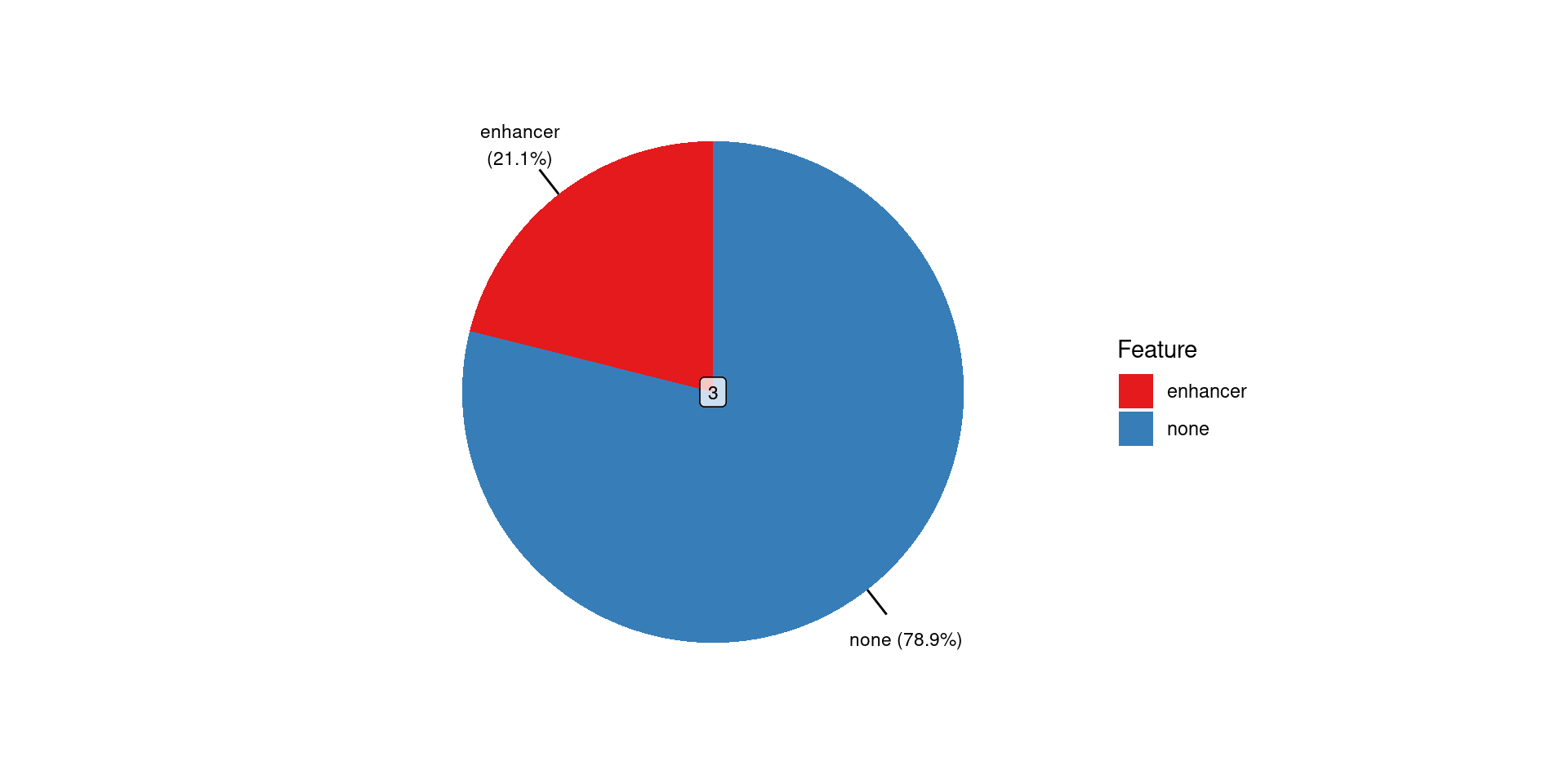
  seqinfo: 1 sequence from GRCh37 genome; no seqlengths

bestOverlap() makes this simple

consensus_peaks$feature <- bestOverlap(consensus_peaks, features, var = "feature", missing = "none")
consensus_peaks

GRanges object with 9 ranges and 3 metadata columns:
      seqnames          ranges strand |    centre         n     feature
         <Rle>       <IRanges>  <Rle> | <numeric> <numeric> <character>
  [1]     chr1   523658-523939      * |    523800         2        none
  [2]     chr1   780837-781330      * |    781141         2        none
  [3]     chr1   821066-821391      * |    821219         2        none
  [4]     chr1   849166-849528      * |    849349         2        none
  [5]     chr1 1707074-1707445      * |   1707252         2        none
  [6]     chr1 1790623-1791019      * |   1790839         2    enhancer
  [7]     chr1 1800936-1801227      * |   1801090         2        none
  [8]     chr1 1814836-1815157      * |   1815023         2        none
  [9]     chr1 1933329-1933586      * |   1933462         2    enhancer
  -------
  seqinfo: 24 sequences from GRCh37 genome

Summarise Binding Patterns

plotPie(consensus_peaks, fill = "feature")

Summarise Binding Patterns

plotPie(consensus_peaks, fill = "feature", scale_by = "width") +
  scale_fill_brewer(palette = "Set1") +
  labs(fill = "Feature")

Differential Binding

`dualFilter()`

Sliding Windows (csaw::windowCounts()) (Lun and Smyth 2014)

Discard non-signal windows using dualFilter()
Combines 1) signal-to-input and 2) overall signal as filtering strategy
Provide regions of expected signal as a guide

GRAVI

Smooth Quantile Normalisation on logCPM (Hicks et al. 2017)
limma-trend (Law et al. 2014)
Range-based \(H_0\) (treat()) (McCarthy and Smyth 2009)

`plotAssayDensities()`

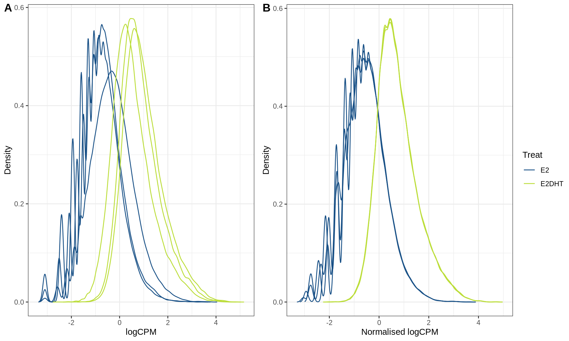
A) Raw logCPM and b) Smooth Quantile Normalised logCPM for the Androgen Receptor (AR)

`plotAssayRle()`

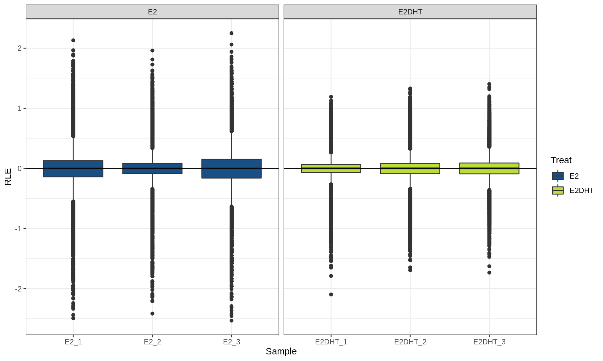
RLE plot calculating RLE within treatment groups

`plotAssayPCA()`

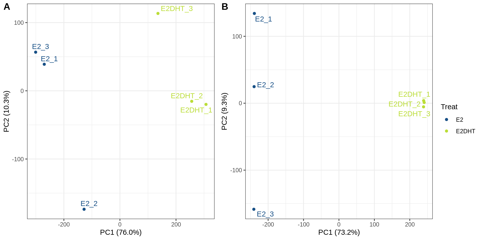
PCA plots A) before and B) after SQN

`mergeByCol()`

Differential binding tested using sliding windows
Merge adjacent sliding windows taking representative window
GRAVI defaults to window with maximum signal
wraps multiple csaw steps
returns representative range

`mergeByCol()`

win

GRanges object with 3 ranges and 3 metadata columns:
      seqnames    ranges strand |   AveExpr     logFC    PValue
         <Rle> <IRanges>  <Rle> | <numeric> <numeric> <numeric>
  [1]     chr1     1-100      * |   4.49781   1.88678 0.0181456
  [2]     chr1    51-150      * |   7.13153   1.61697 0.0128710
  [3]     chr1   101-200      * |   5.92108   1.41863 0.0452510
  -------
  seqinfo: 1 sequence from an unspecified genome; no seqlengths

mergeByCol(win, col = "AveExpr", pval = "PValue")

GRanges object with 1 range and 8 metadata columns:
      seqnames    ranges strand | n_windows      n_up    n_down keyval_range
         <Rle> <IRanges>  <Rle> | <integer> <integer> <integer>    <GRanges>
  [1]     chr1     1-200      * |         3         1         0  chr1:51-150
        AveExpr     logFC    PValue PValue_fdr
      <numeric> <numeric> <numeric>  <numeric>
  [1]   7.13153   1.61697  0.012871   0.012871
  -------
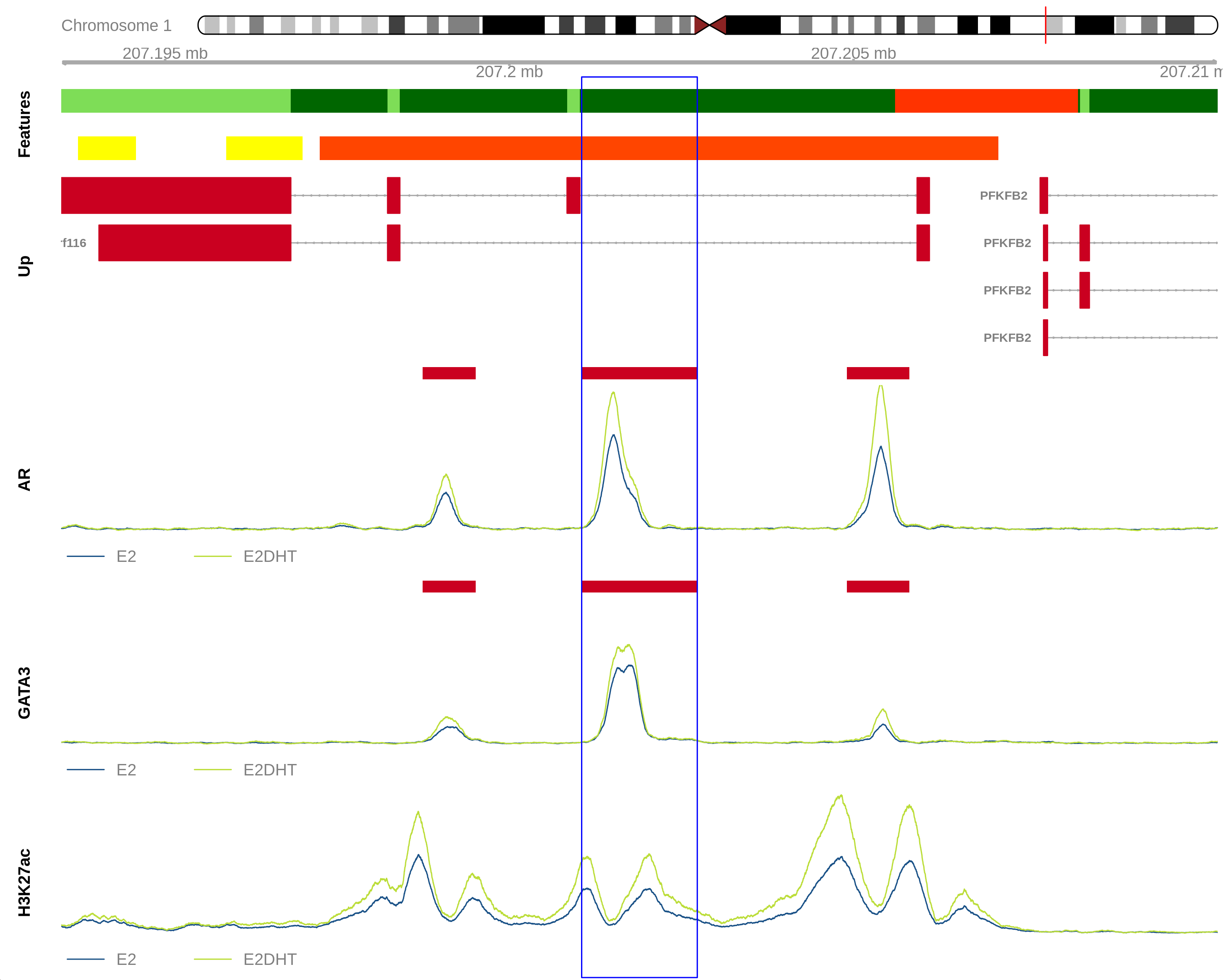
  seqinfo: 1 sequence from an unspecified genome; no seqlengths

`mapByFeature()`

mapByFeature(
  gr,
  genes,
  prom,
  enh,
  gi,
  cols = c("gene_id", "gene_name", "symbol"),
  gr2prom = 0,
  gr2enh = 0,
  gr2gi = 0,
  gr2gene = 1e+05,
  prom2gene = 0,
  enh2gene = 1e+05,
  gi2gene = 0,
  ...
)

`plotProfileHeatmap()`

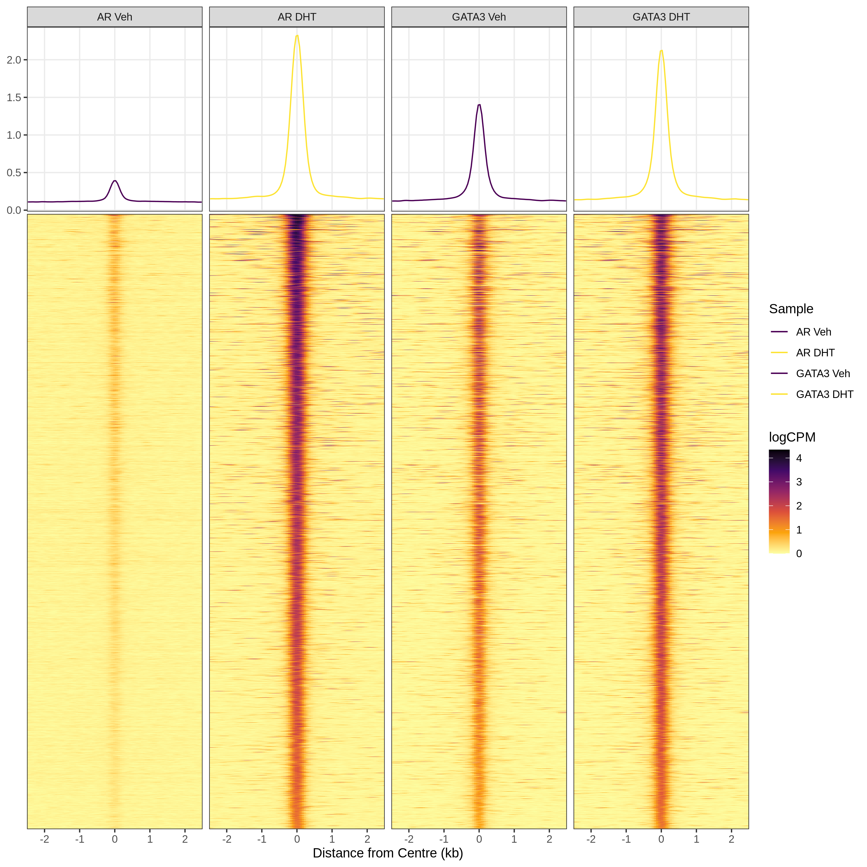
Uses ggplot2 plotting with facets for samples or peak groupings

`plotHFGC()`

Wraps GViz plotting functions
plot optional 1) HiC, 2) Features, 3) Genes or 4) Coverage
Helpful for visualising multiple ranges quickly

References

Blischak, John D, Peter Carbonetto, and Matthew Stephens. 2019. “Creating and Sharing Reproducible Research Code the Workflowr Way [Version 1; Peer Review: 3 Approved].” F1000Research 8 (1749). https://doi.org/10.12688/f1000research.20843.1.

Hickey, Theresa E., Luke A. Selth, Kee Ming Chia, Geraldine Laven-Law, Heloisa H. Milioli, Daniel Roden, Shalini Jindal, et al. 2021. “The androgen receptor is a tumor suppressor in estrogen receptor–positive breast cancer.” Nature Medicine 2021 27:2 27 (2): 310–20. https://doi.org/10.1038/s41591-020-01168-7.

Hicks, Stephanie C, Kwame Okrah, Joseph N Paulson, John Quackenbush, Rafael A Irizarry, and Héctor Corrada Bravo. 2017. “Smooth quantile normalization.” Biostatistics 19 (2): 185–98. https://doi.org/10.1093/biostatistics/kxx028.

Law, Charity W, Yunshun Chen, Wei Shi, and Gordon K Smyth. 2014. “Voom: Precision Weights Unlock Linear Model Analysis Tools for RNA-seq Read Counts.” Genome Biol. 15 (2): R29.

Lun, Aaron T L, and Gordon K Smyth. 2014. “De Novo Detection of Differentially Bound Regions for ChIP-Seq Data Using Peaks and Windows: Controlling Error Rates Correctly.” Nucleic Acids Res. 42 (11): e95.

McCarthy, Davis J, and Gordon K Smyth. 2009. “Testing Significance Relative to a Fold-Change Threshold Is a TREAT.” Bioinformatics 25 (6): 765–71.

Using extraChIPs with GRAVI

Introduction

Who Am I?

GRAVI

GRAVI

GRAVI

GRAVI

extraChIPs

GRAVI

Working With Ranges: tibble Coercion

Working With Ranges: tibble Coercion

Working With Ranges: tibble Coercion

Operations Retaining mcols: reduceMC()

Operations Retaining mcols: reduceMC()

Operations Retaining mcols: reduceMC()

Set Operations Retaining mcols

Tidyverse-inspired Functions: chopMC()

Tidyverse-inspired Functions: distinctMC()

Tidyverse-inspired Functions: distinctMC()

Additional Helpers

Working with Peaks

importPeaks()

plotOverlaps()

plotOverlaps()

makeConsensus()

makeConsensus()

makeConsensus()

makeConsensus()

Map To Features

Summarise Binding Patterns

Summarise Binding Patterns

Differential Binding

dualFilter()

GRAVI

plotAssayDensities()

plotAssayRle()

plotAssayPCA()

mergeByCol()

mergeByCol()

mapByFeature()

plotProfileHeatmap()

plotHFGC()

References

Working With Ranges: `tibble` Coercion

Working With Ranges: `tibble` Coercion

Working With Ranges: `tibble` Coercion

Operations Retaining `mcols`: `reduceMC()`

Operations Retaining `mcols`: `reduceMC()`

Operations Retaining `mcols`: `reduceMC()`

Set Operations Retaining `mcols`

Tidyverse-inspired Functions: `chopMC()`

Tidyverse-inspired Functions: `distinctMC()`

Tidyverse-inspired Functions: `distinctMC()`

`importPeaks()`

`plotOverlaps()`

`plotOverlaps()`

`makeConsensus()`

`makeConsensus()`

`makeConsensus()`

`makeConsensus()`

`dualFilter()`

`plotAssayDensities()`

`plotAssayRle()`

`plotAssayPCA()`

`mergeByCol()`

`mergeByCol()`

`mapByFeature()`

`plotProfileHeatmap()`

`plotHFGC()`